Systemic Immune Profiling: Optimizing Large Plasma Cohorts for Biomarker Discovery

When immune profiling breaks at scale, it's rarely the pathway biology—it's pre-analytics and batch drift. In large plasma cohorts, small inconsistencies compound across centers and months, drowning true signals in plate-to-plate noise. This article distills audit-ready best practices to help immunologists and translational scientists keep systemic error within acceptable bounds, so the biomarkers you report remain reproducible and decision-grade.

Key takeaways

• Treat pre-analytics as the primary source of failure in large plasma cohorts; standardize tube type, processing time, centrifugation, aliquoting, storage, freeze–thaw limits, and shipping.
• Build a QC diagnostics suite: plate/batch NPX distributions, PCA/UMAP clustering, bridge/replicate correlations, internal control flags, and missingness/LOD reports.
• Design for stability: randomize across plates, balance groups, and place bridge samples on every plate to quantify and correct plate effects.
• Correct drift with a documented workflow: diagnose → normalize/bridge → correct (e.g., ComBat or BAMBOO) → re-diagnose. Preserve biology while removing technical variance.
• Make LOD/LOQ policy explicit: define filtering, treatment of <LOD values, and imputation/censoring rules; document thresholds and rationale.
• Keep a one-page checklist with QC triggers and corrective actions. It's your insurance policy during reviews and audits.

Pre-analytics that actually hold under scale for immune profiling

If you get this section right, many downstream "batch-correction" problems shrink. Consistency beats heroics for immune profiling in large plasma cohorts.

• Anticoagulant choice and consistency: EDTA is widely preferred for plasma proteomics and general biobanking; citrate is acceptable for coagulation-focused endpoints; heparin can interfere with some downstream enzymatic assays—use only with validation. Maintain the same anticoagulant across centers to avoid confounding. See the biobanking overview in the ISBER-aligned summary of best practices in the LabKey resource and related SOP literature in biobanking and translational medicine for context: ISBER-aligned biobanking overview and standard biobank SOPs in JoVE. For interference policies and hemolysis, refer to European Federation guidance on HIL indices: EFLM/IFCC HIL interference guidance (2024).
• Time-to-processing and centrifugation: Define site-specific limits for time from collection to first spin (e.g., process within hours) and centrifugation regimes (e.g., 1,000–2,000 × g for ~10 minutes at 2–8°C) to achieve platelet-poor plasma. Document the exact parameters and enforce with training logs.
• Aliquoting and storage: Aliquot to minimize freeze–thaw (FT). Store at −80°C (or colder) with continuous temperature monitoring. Track aliquot histories in your LIMS.
• Freeze–thaw limits: Aim for ≤2 FT cycles for proteins near LOD; design your aliquot volumes accordingly. This is a conservative, example threshold drawn from common biorepository practice and should be validated for your assays.
• Shipping and cold-chain: Ship on dry ice or LN2 vapor with temperature indicators; reject or quarantine shipments that breach the cold chain pending QC review. Maintain chain-of-custody documentation.
• Interference policies: Implement hemolysis, icterus, and lipemia (HIL) indices with reject/accept rules and remediation steps. Standardized HIL handling is widely recommended in clinical laboratory practice; see the EFLM review cited above.

For platform-aware QC visuals (NPX distributions, PCA/UMAP) and standardized normalization tasks, Olink's software documentation provides useful references: Olink NPX Software overview.

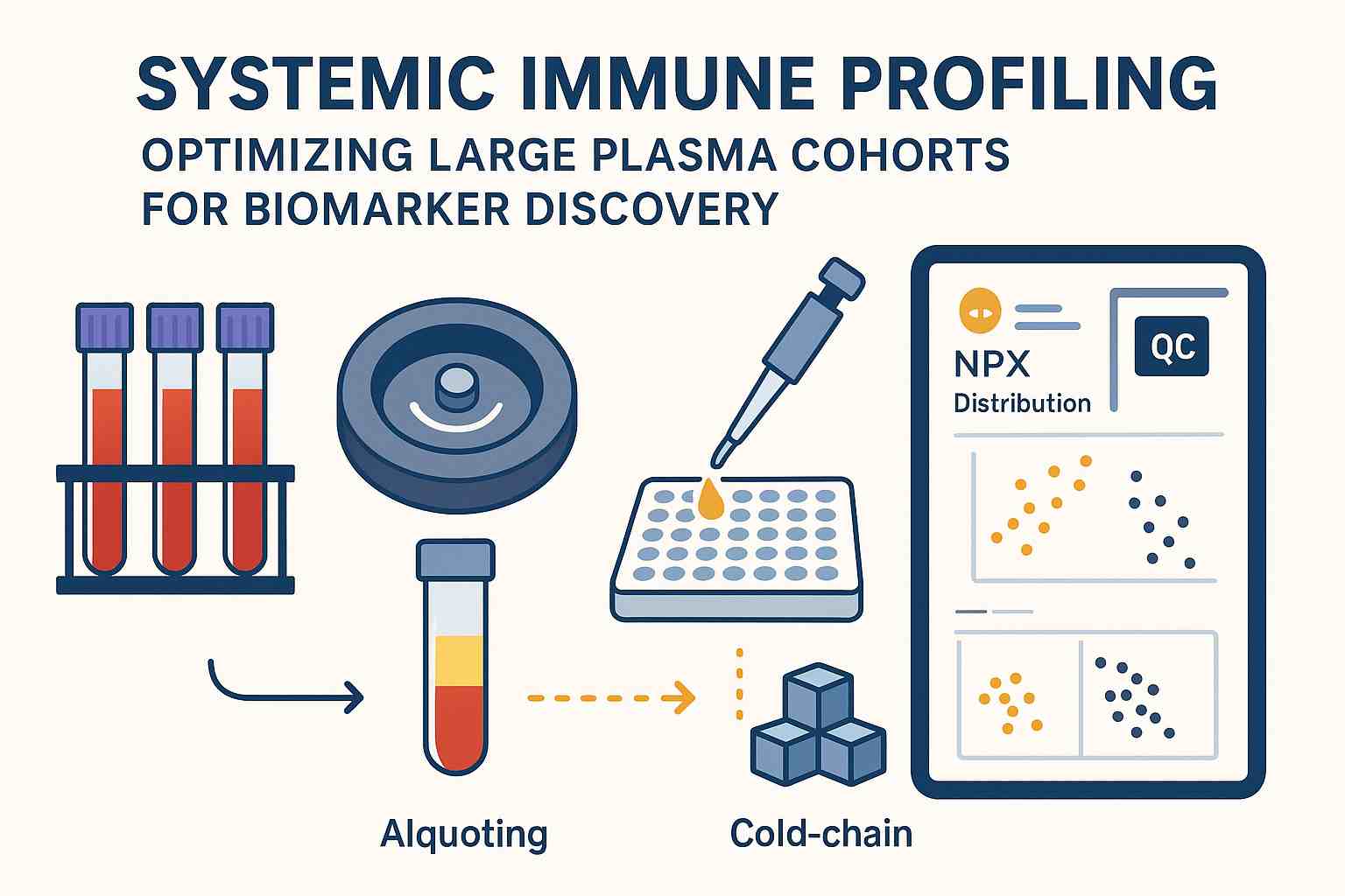
Transforming pre-analytic noise into biological signal.

Unstandardized collection and processing create batch effects that obscure true immune profiles. Implementing rigorous standardization, followed by bridge-sample normalization and stepwise algorithmic correction, restores data integrity and reveals true biological clusters.

QC diagnostics for immune profiling in large plasma cohorts

You can't correct what you can't see. Build a routine set of diagnostics that every batch must pass for immune profiling at scale.

• Plate and batch NPX distributions: Inspect density/violin plots for each plate and batch; large median shifts or heavy tails are red flags. Re-check after normalization.
• Dimensionality reduction: Run PCA/UMAP on the NPX matrix to visualize clustering by plate, lot, or site. Acceptable outcomes show that biology—not plate—is the primary driver of separation after correction. Olink's NPX Software supports these checks: see the NPX Software documentation.
• Replicate and bridge correlations: Compute Pearson/Spearman r for technical duplicates and for bridge samples repeated across plates. After normalization, aim for high correlations (example target >0.95; investigate if <0.90). The platform has demonstrated robust reproducibility in plasma in peer-reviewed work; see the 2022 study by Carlyle and colleagues: reproducibility of Olink panels in plasma (Frontiers in Neurology, 2022).
• Internal control flags: Review vendor-provided internal controls and sample-level QC flags, and define plate failure criteria and re-run rules in your SOPs.
• Missingness and LOD reports: For each protein, report percent above LOD, call-rate, and missingness pattern. Use these stats to inform filtering (e.g., remove proteins with extensive missingness) and to guide LOD-aware modeling downstream.

Bridge-sample blueprint for cohort-scale stability

Bridge (reference) samples transform batch effects from invisible drift into quantifiable offsets.

• What to use: A stable pooled plasma control or a well-characterized biological reference covering a wide NPX dynamic range.
• How many and where: Include bridges on every plate, distributed consistently. Randomize study samples and balance biological groups per plate. For longitudinal designs, where possible, place all timepoints for a participant on the same plate to reduce within-subject technical variance.
• Proportions and power: Many large projects allocate a low double-digit number of reference wells per plate (illustratively 10–12) to ensure robust estimates of plate-specific adjustments. Confirm sufficiency with diagnostics.
• Documentation: Track lot numbers, dates, and well positions for bridges; maintain a changelog when references are replenished.

If you're still finalizing study design and plate layout, see this complementary guide on cohort power and QC strategy: Designing a Large-Scale Proteomics Study with Olink.

Batch and drift correction cookbook

Prevention first; correction second. When you must correct, combine bridging with robust statistical methods, and always re-diagnose.

• Diagnose → Normalize/Bridge → Correct → Re-diagnose: Treat this as a gated process. Do not rush to global correction without confirming plate design and normalization.
• Bridge-based normalization: Use reference samples to compute plate-level offsets, then apply adjustments and re-check drift. Olink's analysis tools and documentation discuss bridging workflows: see Olink Analyze (bridging functions) and UK Biobank PPP materials.
• Algorithmic correction options:
  • ComBat (sva): Effective for known batch covariates with sufficient per-batch size. For recent proteomics context, see the 2024 discussion in J. Proteome Res.: ComBat use in high-throughput proteomics (2024).
  • BAMBOO: A robust regression approach leveraging bridging controls; developed in the context of large Olink datasets (e.g., UKB-PPP) and shown to reduce false discoveries compared to naive methods. See the method description: BAMBOO for PEA batch correction.
  • RUV-based/proBatch/TAMPOR: These frameworks can be effective depending on control structure and study design; always validate that biological signals are preserved via post-correction diagnostics.

Example R-style pseudocode

• Re-diagnose and document: After correction, confirm reduction in plate clustering, improved bridge correlations, and stable NPX distributions. Record software versions, parameters, and plots for audit.

For a population-scale blueprint, review the UK Biobank Pharma Proteomics Project QC materials: UKB-PPP QC companion document.

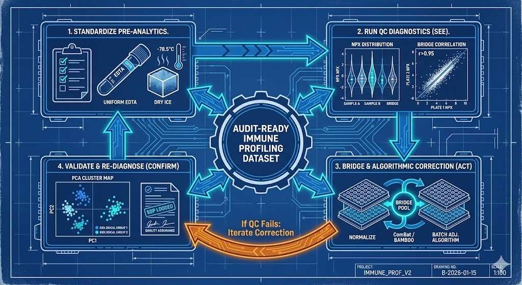The iterative blueprint for audit-ready immune profiling.

LOD/LOQ policy and missing-data strategy in immune profiling

Ambiguity here derails reproducibility. Write down your policy and stick to it.

• Reporting: For each assay, report the fraction above LOD and any available LLOQ/ULOQ. Avoid converting NPX to absolute concentrations without assay-specific calibration. See the Olink documents and LOD tutorials: LOD handling in OlinkAnalyze.
• Filtering: Choose study-appropriate thresholds (e.g., remove proteins with >20% missingness, or require detection above LOD in ≥50–75% of samples). Always justify and pre-register these choices.
• Handling <LOD values: Favor censoring-aware analyses or models that incorporate detection limits rather than naive single-value imputation. If imputation is necessary, perform sensitivity analyses and disclose methods.

Practical execution support

In practice, many teams pair internal SOPs with a partner to operationalize the plan. For example, a vendor can pre-validate EDTA tubes and centrifugation regimes across collection sites, implement pooled-plasma bridges on every plate, and deliver a standard QC packet per batch: NPX distributions, PCA plots, internal control summaries, replicate/bridge correlation matrices, and a change log. This packet makes it straightforward to apply a documented correction pipeline (bridging, then ComBat or BAMBOO where justified) and to re-diagnose before locking the dataset. Partners like Creative Proteomics can also harmonize metadata capture (anticoagulant, freeze–thaw history, storage durations) and provide neutral recommendations when a plate fails (for instance, triggering a re-run if bridge correlation drops below a predefined threshold). The value is not "marketing sparkle" but removing ambiguity and shortening the path to audit-ready data.

Downstream validation and multi-omics tie-in

Immune biomarkers that survive rigorous pre-analytics and QC are stronger candidates for validation and mechanism-building. For study-level planning on cohort size, power, and QC strategy, review this guide: Designing a Large-Scale Proteomics Study with Olink. When moving beyond association toward causality and biological context, consider multi-omics alignment (genomics, transcriptomics) to triangulate signals and support target decisions; see: Integrating Olink Proteomics with Genomics and Transcriptomics.

FAQ

What's the biggest failure mode in immune profiling of large plasma cohorts?

Cross-center batch effects and long-term drift. Biology rarely rescues a poor pre-analytic setup.

EDTA vs citrate vs heparin—does it matter?

Yes. EDTA is widely preferred for plasma proteomics; citrate can be fine for coagulation endpoints; heparin may interfere with some assays. Pick one and keep it consistent across centers; document the choice and validation.

How many bridge samples should I run per plate?

Include them on every plate. A low double-digit number of wells per plate devoted to references (e.g., 10–12) is a pragmatic starting point—validate sufficiency with diagnostics.

How strict should my freeze–thaw policy be?

Design to avoid repeated cycles. A conservative starting point is ≤2 cycles for low-abundance proteins, but validate this for your targets and document exceptions.

Should I always run ComBat or BAMBOO?

No. Diagnose first. If bridging and normalization already remove plate effects (as shown by PCA and bridge correlations), additional correction may be unnecessary. If drift persists, methods like ComBat or BAMBOO can help—re-diagnose afterward to ensure biology is preserved.

What do I do with <LOD values?

Report them transparently. Prefer censoring-aware models or LOD-informed analyses over naive single-value imputation. If you impute, run sensitivity analyses and disclose your method.

How do I handle a problematic plate that clusters separately post-correction?

Check internal controls, review bridge correlations, confirm no cold-chain breach or anticoagulant mismatch, and consider re-running the plate. Document decisions and outcomes.

Next steps

If your cohort is moving from discovery toward validation, tighten pre-analytics, expand bridges, and lock a documented correction workflow for immune profiling. For complex multi-center studies, consider scoping a QC plan with a specialized partner to accelerate audit-ready delivery.

Creative Proteomics can support large-cohort serum and plasma immune profiling through tailored Olink-compatible assay services—see the Olink proteomics assay services page for how these offerings can help standardize sample handling, implement pooled bridge controls across plates, and deliver batch-level QC packets for large cohorts (Olink proteomics assay services). For regulated contexts (e.g., studies informing clinical decisions), have an SME review your QC policies and analysis pipeline before inclusion in submissions.