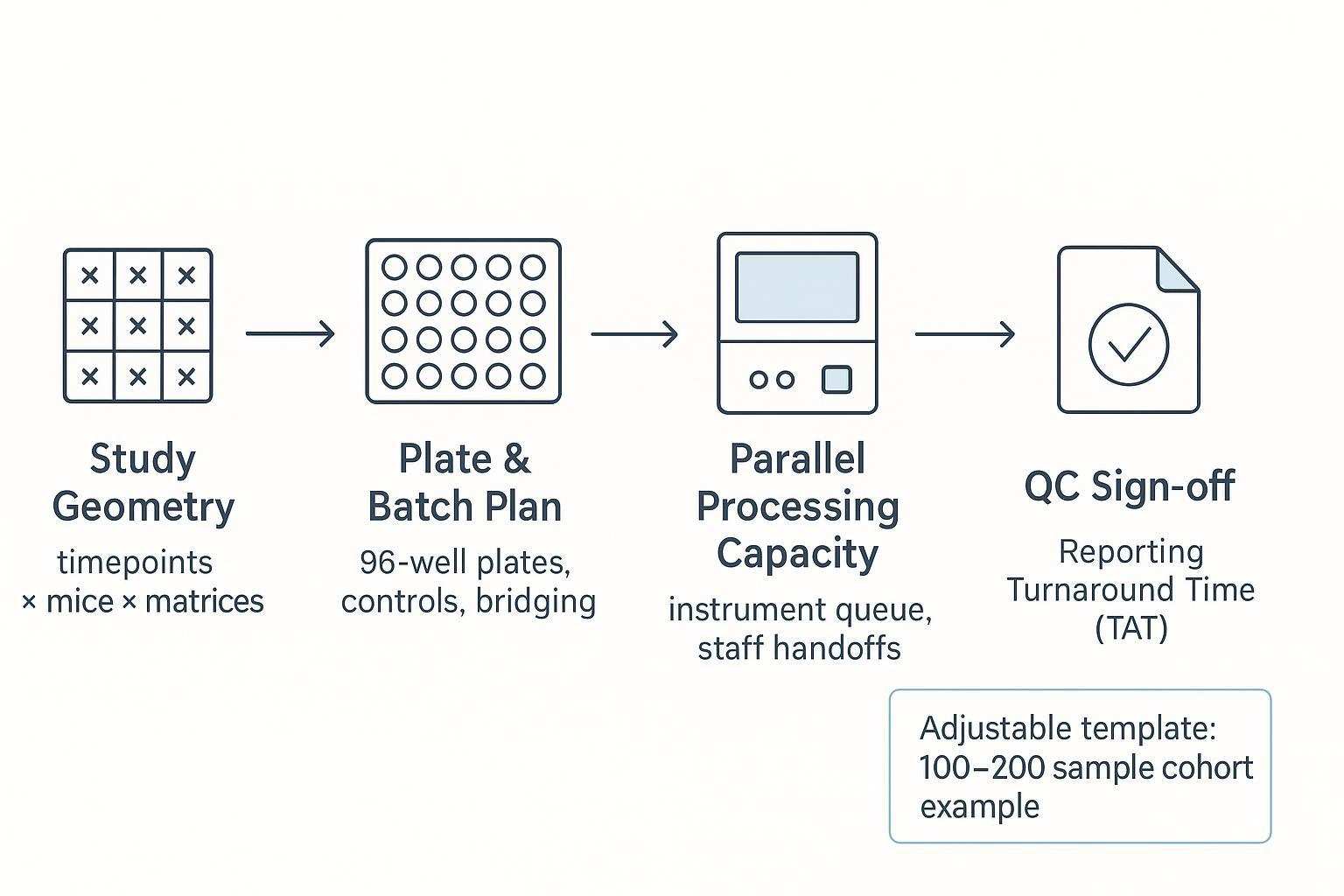
How to Plan Throughput & TAT for Longitudinal Mouse Studies

Planning a longitudinal mouse study with plate-based proteomics is as much an operations exercise as it is a scientific one. This guide translates your study geometry (timepoints × mice × matrices) into plates, batches, queues, QC sign-off gates, and realistic turnaround time (TAT) ranges—so you can make audit-ready decisions without overpromising.

Who this guide is for — understanding throughput and TAT

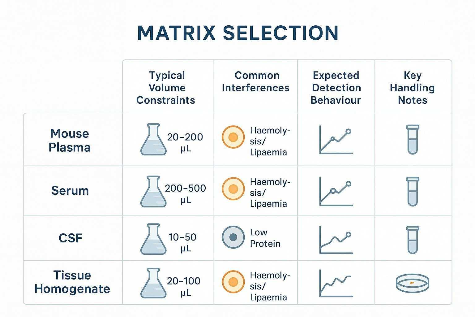
If you lead preclinical or translational work and need reproducible proteomics from limited mouse serum/plasma, read on. By throughput, we mean your effective weekly velocity: how many samples you can move from receipt to post-run QC without compromising comparability. TAT is the total calendar window from sample receipt to report delivery, including explicit QC holdpoints and rerun buffers. We focus on serum/plasma cohorts and use an adjustable mid-size example (100–200 samples) to demonstrate the workflow.

Key takeaways

Build audit-ready longitudinal comparability by using shared bridge samples and explicit QC sign-off gates.
Convert study geometry into 96-well plate math early to expose real constraints on longitudinal mouse study throughput planning.
Model TAT as best/typical/worst ranges with defined QC gates and a rerun buffer instead of a single promise date.
Choose batching strategies by timepoint, by cohort, or hybrid based on drift risk, instrument queue, and analysis needs.
Document decisions and QC outcomes; your audit trail is part of the science.

Step 1 — Map your study geometry — timepoints × mice × matrices

Start by writing down seven inputs in your protocol. Specify the number of mice (typically 40–80), the number of longitudinal timepoints (commonly 3–5), and the primary matrix (serum/plasma). State whether you will include technical replicates at any timepoint. Decide how many wells per plate you will reserve for controls and how many for shared bridge samples to maintain cross-batch comparability. Define your expected rerun buffer (for example, 5–10% of wells) based on historical QC experience. Finally, note instrument run time per plate and staffing shifts, because these drive your queue.

There are pitfalls to avoid in longitudinal designs. Missing timepoints and resampling can bias trajectories; carryover happens when plate position correlates with biology. Randomize positions so biological groups don't map to edges or columns, or block by timepoint when trend integrity is paramount. Confirm serum/plasma handling and volumes against panel requirements before locking the schedule—see the public Olink sample preparation guidelines for collection and storage practices.

Step 2 — Convert study geometry into plates, batches, and queues

Plate math comes first. In a 96-well format, you seldom have 96 true sample wells. Many teams reserve a set of wells for external controls and negatives per plate and add shared bridge samples across batches to support bridging normalization. The UK Biobank pattern often cited allocates triplicate inter-plate controls and negatives, leaving an effective capacity closer to the high 80s once controls and bridges are accounted for; principles are described in the UKB Olink QC companion document (2021).

Now choose a batching strategy for longitudinal mouse cohorts:

Batch by timepoint: Minimizes temporal drift within timepoints and keeps comparisons cleaner; however, it can create queue spikes.
Batch by cohort (subsets of mice): Smooths instrument load and staffing; requires stronger bridging across timepoints.
Hybrid: Mixes both to control drift and balance capacity; demands disciplined bridge sample placement.

When you draft the batch list, align instrument booking with staff handoffs. Bridging normalization practices in the OlinkAnalyze bridging introduction explain why consistent bridge samples per batch matter.

Plate math — 96-well logic, controls, and blanks

Effective throughput depends on the number of usable wells per plate after you reserve external controls (e.g., plate controls in triplicate, negatives in triplicate, pooled precision controls) and bridge samples. Keep 1–2 spare wells per plate if possible to absorb immediate reruns without re-queuing the entire batch. The normalization approach described in Olink's data normalization white paper highlights how inter-plate controls help correct between-plate variability.

Batching strategies for longitudinal projects — by timepoint vs by cohort vs hybrid

Three batching strategies for longitudinal mouse studies—choose based on drift risk, instrument queue, and analysis needs.

Step 3 — Design a plate layout that survives QC and reruns

Place controls and bridge samples deliberately. Distribute blanks, negative controls, and plate controls in positions that expose edge effects and drift across the plate rather than clustering them. Spread bridge samples so you can detect and correct any between-plate shifts later. Randomize sample positions by default to avoid technical position correlating with biology; block by timepoint only when it improves interpretability.

Edge-effect mitigation is practical and publishable. Control humidity, use appropriate seals/covers, and avoid leaving the outer wells disadvantageously empty. Manufacturer notes outline mitigations for optical assays; for example, see Eppendorf's edge-effect application note and Agilent's evaluation of edge effects .

Control placement rules — edge effects, drift detection, bridging

96-well plate layout with controls and bridging samples Example 96-well plate discipline for longitudinal projects: distributed controls and bridging samples to support cross-batch comparability.

Randomization vs blocking — when each matters

Randomize to break correlations and enable robust NPX normalization; block by timepoint when trend analysis across visits is the primary scientific question. Whichever you choose, document your rule and rationale in the protocol. For normalization context (IPC triplicates, intensity normalization), see Olink's normalization white paper.

Step 4 — Longitudinal mouse study throughput planning — estimate with parallel processing

Here's the deal: much of sample prep can run in parallel, but incubation, extension, amplification, and readout steps form the critical path. Build a per-plate time budget that distinguishes parallelizable tasks (prep, initial data QC) from sequential gates (assay run and readout). Capacity planning should account for instrument slots, lanes/flowcells if applicable, and staff handoffs.

Define your weekly velocity by counting plates per week times the effective wells per plate after controls and bridges. Then pressure-test the schedule against booking policies and realistic QC review times. Olink's workflow materials and blog give qualitative guardrails on where the bottlenecks occur; for a deeper understanding of parallelization benefits in proteomics operations generally, see the high-throughput QC framework in "A framework for quality control in quantitative proteomics" (2024) .

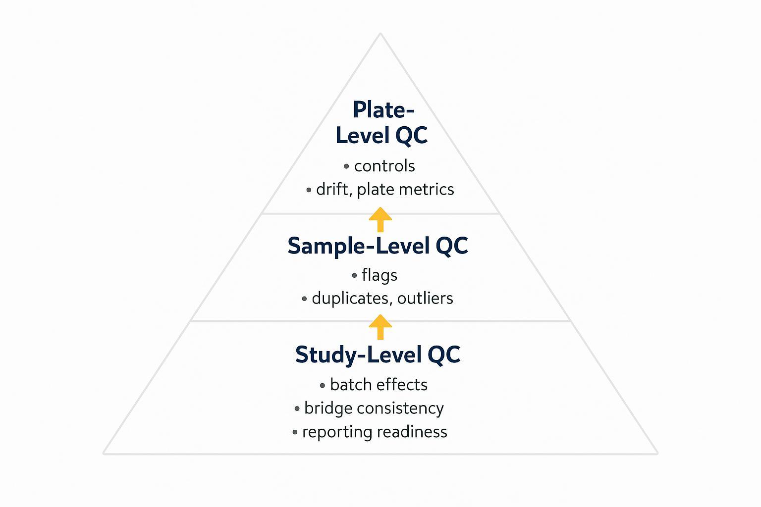
The critical path — what gates your timeline

Sequence the steps that must occur in order and highlight QC gates where the schedule can slip. Your critical path typically runs: sample receipt → assay run/readout → primary QC → normalization/bridging → bioinformatics QC → reporting. Document handoffs by role to prevent stalls.

Capacity planning — instruments, lanes/flowcells, staff handoffs

If your readout instrument has limited slots or specific run lengths, anchor batch sizes to those constraints. Stagger prep so plates land at the readout queue with minimal idle time, but don't compress QC review windows. Clear role assignment reduces ambiguity.

Step 5 — Build a realistic TAT window — best-case, typical, worst-case

Express TAT as a range with explicit QC sign-off gates rather than a single date. Define holdpoints: Sample Receipt QC, Pre-run System Suitability, Post-run Plate QC, and Pre-report Sign-off. Best-case assumes everything passes the first time; typical includes minor reruns; worst-case includes one batch-level rerun or holiday/weekend delays.

Add a rerun buffer to your calendar math—plan enough spare wells or time to re-queue a subset without derailing the schedule. For normalization and QC documentation practices (IPC, LOD handling, intensity vs bridging normalization), see the public Olink data analysis process .

Gantt timeline for throughput and QC sign-off turnaround time A realistic TAT window is driven by the critical path and QC gates—this timeline shows what runs in parallel vs what must happen sequentially.

Step 6 — Contingency planning — weekends, holidays, shipping, sample failures

Plan for calendar exceptions and logistics. Weekends and holidays extend TAT unless you pre-book instruments and staff shifts; avoid shipping over weekends; maintain cold-chain integrity end-to-end. If a temperature logger shows a breach, quarantine affected samples, review stability guidance, and document decisions in the QC log. Reserve spare wells or a small batch slot for rapid reruns.

Worked example — adjustable mid-size cohort (100–200 samples)

Let's map a common scenario and show the swap-in template flow.

Example inputs and plate plan: 50 mice × 4 timepoints = 200 serum/plasma samples; no technical replicates; reserve 8 external control wells per plate (triplicate inter-plate controls, triplicate negatives, duplicate pooled precision); include 2–4 shared bridge samples per batch; rerun buffer = 5–10%.

Derived outputs: At an effective capacity of ~88 sample wells before bridges, you'll likely run 3–4 plates for 200 samples depending on bridge allocation. A hybrid batching approach might run two plates in week 1 and one to two plates in week 2, balanced against instrument bookings. The template auto-calculates: total plates, batches, queue dates, QC gates, and best/typical/worst TAT windows.

Swap-in template — adapt to your sample count

Inputs block: number of mice; number of timepoints; technical replicate policy; controls per plate; bridge sample strategy; rerun buffer; instrument run time/plate; staff shifts per week.

Outputs block: total samples; plates and batches; queue schedule; QC gate dates; best/typical/worst TAT range.

FAQ — high-intent questions before committing

How many samples per week can you realistically process?

Your weekly throughput equals plates per week × effective wells per plate after controls and bridges. For many Olink-style 96-well runs, this means planning on the high 80s per plate, then subtracting bridge wells you allocate. Velocity depends on batching strategy and QC pass rates.

What's the expected TAT once QC is included?

Model a range with explicit gates: best-case (no reruns), typical (minor reruns and standard review windows), worst-case (one batch-level rerun or calendar delays). Anchor the schedule to the critical path and keep QC documentation audit-ready.

Can you handle rush? What changes, what costs more?

Rush options are possible: priority queue slots, weekend staffing, and smaller batch sizes reduce idle time. Trade-offs include higher cost and tighter coordination. No hard promises—rush feasibility depends on queue status and QC guardrails at the time you request it.

Request a scheduling template — conversion and next steps

What you'll receive: an editable scheduling template (Gantt-style) that translates your study design into plates, batches, QC gates, and a defensible TAT range, plus a simple plate blueprint.

What we need from you: your inputs checklist (mice, timepoints, matrix, replicates policy, controls/plate, bridge plan, rerun buffer, instrument run time, staffing). Upload via the request link/button.

Scheduling template preview for longitudinal sample throughput and TAT Request an editable scheduling template to translate your study design into plates, batches, QC gates, and a defensible TAT range.

Throughput & TAT Planning for Longitudinal Mouse Studies (Step-by-Step Guide)