
Why Data Processing Makes or Breaks Your Olink Results
In proteomics research, raw numbers are only as useful as your data pipeline's rigor. One mis-step in normalization or quality control (QC) can turn a promising cytokine signature into noise. Recent studies using Olink proteomics have shown that batch effects or uncontrolled variation often dominate biological signal—masking real differences. If your lab or CRO lacks a firm grasp on the data processing flow, you risk false leads, wasted time, and lost funding.
The real power of Olink assay-based discovery lies not just in high multiplexing, sensitivity, or small sample volume—but in turning raw readouts into reliable insights. From Normalized Protein eXpression (NPX) to handling non-detects, correct QC, normalization, and downstream statistics are what separate reproducible outcomes from ambiguous ones.
In this article, we guide you through the advanced data analysis process behind Olink proteomics (especially cytokine panels). You'll learn how raw readouts become trustworthy data you can interpret, reproduce, and act upon.
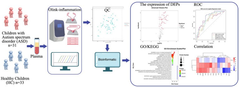 Figure 1. Study strategy and schematic illustration of plasma Olink proteomics.
What Is NPX — The Foundation of Olink Proteomics Analysis
To derive meaningful scientific insights from Olink proteomics data (including Olink Cytokine Panels), understanding Normalized Protein eXpression (NPX) is essential. It is the core unit upon which QC, normalization, and downstream statistics are built.
Definition & Purpose of NPX
NPX is Olink's relative quantification unit, expressed on a log₂ scale. A higher NPX → higher protein abundance in your sample.
NPX is not an absolute concentration (e.g. pg/mL) but a measure of relative change, making it ideal for comparing samples within the same experimental project.
Because of NPX's nature, comparisons across different projects or batches require bridging or reference samples (see later sections). Direct NPX comparisons without such normalization may lead to misleading conclusions.
How NPX Is Calculated (qPCR-Readout Panels)
For the Olink Target 96 / 48 panels, which use qPCR readout, NPX calculation involves several steps designed to remove technical variation. The white paper "Data Normalization and Standardization" outlines this process.
Ct Values: The qPCR produces cycle threshold (Ct) values for each analyte (protein). A lower Ct = more initial template (thus more protein).
Extension Control Adjustment: Each analyte's Ct is compared to an internal "extension control" to generate a delta Ct (dCt). This adjusts for variation in extension and amplification/detection steps.
Inter-Plate Control (IPC): The dCt is then normalized with respect to an inter-plate control sample (run in multiple plates) to adjust for plate-to-plate variation, producing a delta-delta Ct (ddCt) structure.
Correction Factor & Inversion: A correction factor, predetermined during panel validation, is applied. The scale is inverted so that higher NPX corresponds to higher protein signal (i.e. so NPX increases as measured protein increases). Hence, NPX = CorrectionFactor − ddCt.
NPX in NGS Read-out / High-Throughput Panels
For Olink panels using NGS as the readout (e.g. Explore / Reveal libraries), NPX is similarly used as a log₂, relative quantification unit. While the upstream readout (sequencing counts) differs from qPCR, the fundamental goal remains: reduce technical variation, enable comparisons within projects.
The software pipelines (e.g. NPX Map, NPX Manager) automatically translate raw counts / sequencing output into NPX values. They include pre-processing steps, internal controls, detection of outliers etc.
Key Properties & Implications of NPX
Since NPX is in log₂, a difference of 1 NPX ≈ a doubling of protein expression, all else equal. Always check which panels or assays this applies to.
NPX values for the same protein across experimental samples are comparable; NPX values for different proteins are not directly comparable in magnitude (because each protein's assay has its own efficiency, dynamic range etc.).
NPX is useful for detecting relative changes (fold changes, trending, expression patterns) rather than absolute quantitation. If absolute concentration is needed, Olink sometimes provides pg/mL values (often for certain panels or upon request) but this comes with limits of quantification considerations.
Summary & Takeaway
Understanding NPX is not optional — it's foundational. Without knowing how NPX is generated and what it can (and cannot) tell you, downstream interpretations (differential expression, clustering, biomarker signature) risk being flawed. The next sections build on NPX to show how QC, normalization, and statistical tools leverage this unit to transform raw data into robust insights.
QC: Internal Controls, Outliers & LOD in Olink Cytokine & Proteomics Panels
Quality control (QC) is essential for trustworthy Olink proteomics analysis. In this section, we break down the built-in controls, how outlier samples are flagged/removed, and how Limit of Detection (LOD) is defined and handled.
Internal & External Controls
To monitor technical performance and sample quality, Olink includes several controls:
| Control Type | Purpose | How It's Used |
| Incubation control (two, non-human proteins) | Tracks the immuno-binding step and overall immunoreaction consistency. | |
| Extension control | Monitors the extension and hybridization steps (independent of target binding). Also used in NPX normalization. | |
| Detection control | Verifies performance of the detection stage (e.g. PCR amplification or NGS detection) to catch errors or drift. | |
| Inter-plate control (IPC) | External pooled sample on each plate to adjust for plate-to-plate variation. Supports data comparability across multiple runs. | |
| Negative control | Background signal (buffer + all reagents, without sample target) to establish baseline noise and help compute LOD. |
Outlier Detection & Sample QC
Outlier detection helps prevent abnormal samples from skewing results. Common practices include:
QC Warnings for Individual Samples: Samples whose internal control signals (Incubation or Detection) deviate too far from the plate median are flagged. For example, if the control value is more than ±0.3 NPX from the plate median, they may receive a QC Warning.
Plate QC Criteria: Entire sample plate runs are evaluated based on the consistency of internal controls' standard deviations. If the run exhibits too much variation (e.g. SD above thresholds), data may be flagged or excluded.
Visualization Tools: Use PCA plots, distance/median-IQR (interquartile range) vs median NPX plots to detect sample outliers across many proteins. These methods are part of the OlinkAnalyze R package.
Removing Proteins with Excess Missing or Below-LOD Values: In some large cohort studies, proteins for which a high proportion of samples fall below LOD or produce QC warnings are removed (e.g. ≥50%) to avoid unreliable analyses.
Limit of Detection (LOD): Definition & Handling
Understanding LOD is vital for handling low-abundance proteins and interpreting missing values.
How LOD is Defined: For each assay and plate, LOD is typically computed using negative control wells. The background signal plus three standard deviations gives the LOD cutoff. The standard deviation is assay-specific and derived from panel validation.
Plate-Specific vs Fixed LOD:
- Plate-Specific / Negative-Control LOD (NC LOD): Calculated using negative controls within the current plate or project. Best when you have enough negative controls and when sample conditions match the experimental design
- Fixed LOD: Pre-computed LOD values released by Olink (based on reference reagent batches) used when project-specific negative controls are insufficient.
Treatment of Values Below LOD:
Some datasets mark them as missing values when they are below LOD and/or QC warnings.
Other analyses include values below LOD, especially when doing biomarker discovery or comparing groups, with appropriate caveats—these data tend to cluster near the LOD and may not severely bias results if handled properly.
Example from Recent Literature
In Technical Evaluation of Plasma Proteomics Technologies (2025), researchers used Olink NPX data and did the following:
- Filtered for values above LOD after performing sample QC and assay QC.
- Treated values below LOD as "missing" to avoid noise from low signal.
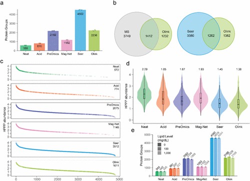 Figure 2. Average number of protein groups identified across five technical replicates. For Olink, protein IDs were reported for assays that were above LOD.
Summary & Key Recommendations
Always include all internal and external controls in the analysis; monitor both sample-level and plate-level QC metrics.
Use visualization (PCA, IQR-vs-median etc.) to spot outlier samples.
Define LOD using negative controls per plate when possible; otherwise use fixed LOD with caution.
Decide ahead of analysis how to handle values below LOD (remove or include conditionally), especially for proteins with many low values.
Normalization Methods: From Within-Plate to Cross-Project Bridging
To extract reliable biological signals from Olink proteomics analysis, normalization is essential. This section covers the major normalization strategies—within-plate, intensity, and bridging—used to correct for systematic technical variation.
Within-Project Normalization Methods
These are methods applied when all samples are within the same project (e.g. same plate(s), same reagent lot etc.).
| Method | When to Use | What It Does / How It Works |
| Plate Control Normalization | Projects with a single plate or when experimental design keeps plates under tightly controlled conditions (e.g. Explore HT single-plate runs). | Adjusts NPX values by using internal controls on each plate to account for plate-to-plate variation. Ensures consistency across plates within one project. |
| Intensity Normalization | Multi-plate projects where samples are randomized across plates. | Assumes all samples are fully randomized; uses global sample intensity distributions to normalize across plates. Helps correct batch effects within a project when plates differ in sample content or handling. |
Bridging: Between Datasets / Projects
When you need to combine data across multiple NPX projects (different plates, batches, or even different Olink product lines), bridging enables comparability. Without bridging, NPX values from different projects are not directly comparable.
Key Concepts in Bridging
- Bridging Samples: Overlapping samples (same biological sample) run in multiple projects, used to compute adjustment factors. These must pass QC and preferably have high detectability (few values below LOD).
- Bridgeable Assays: Only certain assays (proteins) that behave similarly across datasets (similar NPX distribution, detection rates etc.) are suitable for bridging. Other assays may need exclusion or separate handling.
Bridging Methods
| Method | What It Does | When to Use |
| Median-Centered Adjustment ("Bridge Normalization") | Compute the median of the paired NPX differences in bridging samples and shift NPX values in non-reference project accordingly so their distributions align. | When datasets have overlapping samples and similar assay behavior; when distribution differences are moderate. |
| Quantile Smoothing / Quantile Normalization | Align entire NPX distribution shapes across projects by smoothing or mapping quantiles based on overlapping sample distributions. Adjusts both central tendency and distribution tails. | Useful when distribution differences are larger or when you want to align more than just median shifts. Often used along with median centering to produce two candidate normalized datasets (and then choose best suited). |
Combining Projects (Within-Product & Between-Product Bridging)
Within-Product Bridging: Projects using the same Olink product (e.g. Explore 3072), but run in different times / labs / plates. Bridging aligns NPX among those.
Between-Product Bridging: When combining data from different Olink product lines (e.g. Explore 3072 with Explore HT or Reveal). Here, overlapping assays across products are used for bridging. Not all assays overlap, and some may not be bridgeable. The bridging methods above (median centering, quantile smoothing) are applied.
Practical Considerations & Workflow
Selection of Bridge Samples:
- Must pass QC.
- Have high detectability (i.e. few proteins below LOD).
- Should cover the dynamic range of NPX values. Avoid selecting only high or only low expressors.
Recommended Number of Bridge Samples:
Varies by platform. Some examples:
Target 96: 8-16 bridge samples
Explore HT: 16-32
Explore 3072 → Explore HT bridging: 40-64 samples
Evaluate Post-Bridge Quality: Use diagnostic plots (PCA, NPX distributions, density plots) to verify whether bridging has aligned datasets without over-correcting or distorting biological variation. If some assays still diverge badly, consider excluding them.
Software Tools: The OlinkAnalyze R package supports functions like olink_normalization(), olink_normalization_bridge(), olink_normalization_n() for applying these normalization and bridging strategies.
Data Transformation & Handling Non-Detects (Below LOD)
When processing Olink proteomics data (especially those involving cytokine panels), how you transform NPX values and deal with measurements below the Limit of Detection (LOD) can strongly affect downstream analyses. In this section, we cover recommended approaches and trade-offs.
Transformation of NPX Data
Proper transformation helps with statistical modelling, visualisation, and comparing across proteins/groups.
NPX values are already on a log₂ scale, which tends to compress large fold-changes and improves symmetry. Therefore, many downstream analyses (e.g. clustering, PCA, linear models) work directly on NPX without further log transformation.
If combining NPX with external data in absolute concentration units (e.g. pg/mL), be cautious: since NPX does not measure absolute quantity directly, merging such data may introduce scale mismatches unless well calibrated.
Some visualisation tools may require scaling or centring (e.g. subtracting sample/plate median, Z-score per protein) to highlight relative changes rather than absolute NPX differences
Estimating Limit of Detection (LOD)
Understanding where LOD is used is critical before deciding how to treat data below it.
Use the OlinkAnalyze R package's function olink_lod() to add LOD values to NPX datasets. It can calculate LOD using negative controls (NC-LOD) or fixed LOD values provided by Olink reference documentation.
For datasets with ≥10 negative controls that pass sample QC, NC-LOD is preferred because it's specific to the plate and batch.
When fewer negative control wells are available (e.g. small pilot studies), using fixed LOD values is acceptable, but these are less precise for that specific project.
What to Do With Values Below LOD
Proteins with measurements under LOD ("non-detects") are common with low-abundance cytokines. How you handle them depends on study design, statistical assumptions, and how much missingness you have.
| Strategy | Pros | Cons / Considerations |
| Include actual values below LOD | Maintains maximal data; better for large studies; may improve statistical power when low vs high abundances differ between groups. | These values may lie in the non-linear, less reliable region of measurement curves. Might bias fold-changes or effect sizes (because one NPX difference in low region may not equal 2-fold change) if interpreted like linear regions. |
| Replace below LOD with a fixed substitute (e.g. LOD or LOD/2) | Simple and easy to implement; retains all proteins in analysis. | Truncates lower tail of NPX distribution; can distort variance estimates; may bias mean or group comparisons. |
| Impute non-detects (statistical imputation) | More sophisticated; can model distribution of low values; may preserve variance and avoid extreme bias. | Requires assumptions about the distribution of data below detection; complex to validate; may distort if assumptions are wrong. |
| Exclude assays with many non-detects | Simplifies analysis; avoids noise from barely detected proteins. | Risk losing potentially biologically relevant proteins, especially low‐expressors; may reduce scope of discovery. |
Best Practices & Recommendations
Assess proportion of measurements below LOD per protein and per group before selecting a handling strategy. For example, proteins with >50% values below LOD may need a different treatment (exclusion or special modeling). (UK Biobank data uses such filters).
Document which strategy you used when you report results. This includes whether you used NC-LOD or fixed LOD, what substitution or imputation you used, or which assays were excluded.
When using parametric statistics (e.g. linear models), test whether including non-detects biases residuals or variance. If so, consider non-parametric alternatives or two-part models (e.g. mixture of detection vs non-detection plus continuous modeling for detected).
Visualise distributions (e.g. density plots, violin plots) including non-detects to see whether zero-censoring or truncation creates artefacts.
Example from Olink Analyze / UK Biobank
The olink_lod() function in the OlinkAnalyze R package adds both PCNormalizedLOD and LOD columns to datasets, depending on whether Plate Control or Intensity normalization was used. Sites often use NC-LOD in large studies.
In UK Biobank's proteomics data, assay‐level results include olink_limit_of_detection for each plate. Researchers filter NPX data using this (e.g. retaining only results > LOD) to ensure detectability.
Summary & Key Takeaway
Handling data transformation and non-detects correctly is as important as QC or normalization. The decisions you make at this stage (whether to include below‐LOD values, how to impute, whether to exclude assays) can meaningfully shape conclusions. For robust Olink proteomics analysis, always:
- Use well‐defined LOD values (NC-LOD or fixed),
- Choose transformation / substitution / imputation consistent with study size and data missingness,
- Evaluate impact of below-LOD values via sensitivity analyses,
- Fully report methods so readers can judge reliability.
Statistical & Exploratory Analyses: From PCA to Differential Protein Expression
Robust Olink proteomics analysis turns NPX matrices into testable biology. In this section, we cover unsupervised exploration (PCA/UMAP, clustering), supervised testing (t-tests/ANOVA, linear mixed models), effect sizes, and multiple-testing control—using tools purpose-built for Olink assay data, including the OlinkAnalyze R package. Cytokine datasets (e.g., Olink Cytokine Panel) benefit from the same workflow with attention to sparsity and LOD handling.
1) Unsupervised exploration: PCA, UMAP, clustering
- Goal: detect batch effects, outliers, and dominant biology before hypothesis tests.
- How: olink_pca_plot() and olink_umap_plot() on QC-filtered NPX; review loadings and sample separation; pair with distance/IQR plots for outliers.
- Tip: scale per-protein if variances differ widely; re-run after removing flagged samples.
2) Group comparison & covariates
Pick statistics to match design and sample size:
- Two groups: olink_ttest() (Welch) or olink_wilcox() for non-parametric.
- >2 groups: olink_anova() with planned post-hoc contrasts (olink_anova_posthoc()).
- Repeated measures / multi-factor designs: olink_lmer() (random intercepts; fixed covariates for age, sex, site, plate). Document contrasts and random-effects structure.
3) Multiple testing & effect sizes
- Control false discoveries with Benjamini–Hochberg FDR; report both raw p and FDR-adjusted values.
- Always pair p-values with effect sizes (NPX mean differences or model coefficients). Use volcano plots to combine both. OlinkAnalyze includes helpers for volcano and heatmap visualisation.
4) Model hygiene: covariates, batch, and intensity
- Include known biological covariates (age, sex, BMI) and technical factors (plate, run, shipment) in your design matrix or as random effects.
- For multi-plate projects, verify normalization first (plate/intensity normalization; bridging when combining projects) and then model residual batch. UK Biobank guidance shows plate IDs and LOD tables joined to NPX before filtering and testing.
5) Visual analytics that matter
- Volcano: highlight FDR-significant proteins with minimum effect size threshold.
- Heatmaps: cluster significant proteins and samples; annotate groups/covariates.
- Pathway enrichment: run olink_pathway_enrichment() on significant proteins to move from lists to biology.
6) Recommended end-to-end recipe
- PCA/UMAP + QC plots → remove outliers; confirm no gross batch.
- Confirm LOD strategy; filter per protein if detectability is poor.
- Choose model (t-test/ANOVA/mixed model) with covariates; fit per protein.
- Adjust FDR; compute effect sizes; visualise (volcano, heatmap).
- Enrich pathways; summarise biologically coherent modules.
7) Case studies (methods you can emulate)
- Population-scale NPX analysis: The UK Biobank Pharma Proteomics Project describes joining per-plate LOD tables to NPX, filtering, then running downstream statistics—an approach you can mirror for large projects. (UK Biobank Documentation, 2023–2024.) (DOI not applicable; technical doc.)
- Disease-focused Olink panel with DE testing and ROC: An Olink Target 96 Inflammation study compared ASD vs controls, used OlinkAnalyze for differential expression, and validated signatures with ROC and enrichment—illustrating a clean NPX→DE→pathway flow. (Zhao et al., 2023. DOI: https://doi.org/10.3389/fnmol.2023.1185021).
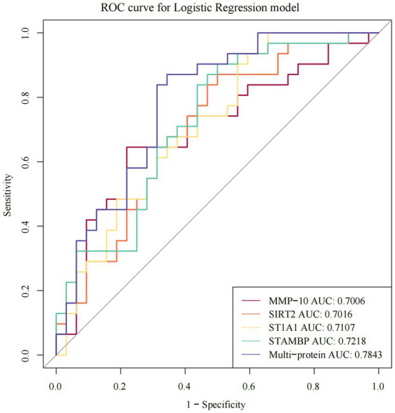 The ROC curves of individual and multi-protein
- For hands-on commands, see the OlinkAnalyze vignette: PCA/UMAP, t-tests, ANOVA, lmer, volcano/heatmaps, and pathway tools are covered with examples.
Natural follow-ups inside your ecosystem
If you're new to the platform fundamentals, skim "Introduction to Olink Proteomics: What You Need to Know" to align assay mechanics with analysis choices. When integrating data from different formats, "Exploring the Olink 96 and 48-Plex Panels: Key Differences" helps you anticipate cross-panel quirks. And if your dataset focuses on immune biology, "Using Olink's Cytokine Panels for Immune System Research" offers context for interpreting cytokine shifts.
Visualization & Biological Interpretation: Pathways, Heatmaps, Biomarker Discovery
Turning NPX tables into biology is where Olink proteomics analysis pays off. In practice, you'll map significant proteins to pathways, visualise patterns with heatmaps/volcano plots, and assemble coherent biomarker stories—especially for immune-focused datasets from the Olink Cytokine Panel and related Olink assay platforms. Below is a practical, research-only workflow anchored in reproducible tools and recent literature.
1) From protein lists to pathways (ORA/GSEA)
Use over-representation analysis (ORA) when you have a clean list of significant proteins; use GSEA when you prefer ranking by effect size or model coefficients.
The OlinkAnalyze R package implements both approaches against MSigDB gene sets via olink_pathway_enrichment(), returning FDR-adjusted pathways plus helper plots.
Good practice
Keep the full, ranked table (statistic + direction) for GSEA.
Verify identifier mapping (gene symbols vs UniProt) before enrichment.
Report pathway size cut-offs and multiple-testing method in Methods.
2) Visual analytics that reveal structure
Volcano plots: Pair FDR with a minimal effect size (e.g., |ΔNPX| ≥ 0.3) to avoid "tiny-but-significant" hits dominating the narrative. olink_volcano_plot() standardises this step.
Heatmaps: Cluster significant proteins and samples; annotate groups, batches, and covariates. olink_heatmap_plot() provides consistent theming, while olink_pathway_heatmap() summarises enriched pathways across contrasts.
Pathway bar/strip charts: Summarise top pathways by Normalised Enrichment Score (NES) or FDR via olink_pathway_visualization().
3) From pathways to mechanism: immune panels as an example
Cytokine-centric studies often enrich cytokine–cytokine receptor interaction, TNF, IL-17/NOD-like receptor, or NF-κB signalling—classic outputs when analysing inflammation with Olink panels. In an ASD plasma study using the Olink Inflammation panel, the authors performed DE testing, GO/KEGG enrichment, and visualised heatmaps/volcano plots to connect NPX signals with immune pathways. (Zhao et al., 2023. DOI: https://doi.org/10.3389/fnmol.2023.1185021).
Larger NPX projects follow similar logic at scale: per-plate LOD tables and metadata are merged prior to testing and enrichment, ensuring downstream pathway calls aren't driven by detectability artefacts. (UK Biobank Olink documentation.)
4) Case study templates you can emulate
Placental-mediated FGR (Explore-384 Inflammation): 225 DE proteins were identified; GO/KEGG enrichment implicated placental vascular function and immune regulation, with model-based selection of key markers—illustrating a robust NPX → DE → enrichment → interpretation chain. (Zhou et al., 2025. DOI: https://doi.org/10.3389/fimmu.2025.1542034).
Comparative platform context: Olink white papers and vignettes detail visual QC, bridging criteria, and enrichment utilities that help separate biological signal from platform effects when reporting figures.
5) Reporting standards for figures & pathway claims
Always state: enrichment method (ORA or GSEA), background set, version of MSigDB, FDR procedure, and effect-size thresholds used for ranking.
Provide full supplementary tables for: protein stats, pathway hits (ID, description, size, NES, FDR), and figure code versions (package + commit/tag).
6) Quick, repeatable recipe
- Start with QC-filtered, normalised/bridged NPX and a pre-registered contrast.
- Run DE with covariates; export ranked tables.
- Enrich with olink_pathway_enrichment(); visualise with pathway bar/heatmap helpers.
- Cross-check enriched pathways against heatmaps of member proteins; inspect redundancy and directionality.
- Translate to biology: relate modules to known immune axes; propose validation assays or orthogonal readouts (research-only).
Integrating Multiple Panels / Datasets: Best Practices
Combining Olink NPX datasets unlocks power at scale, but invites bias. Treat integration as a design problem first, then an algorithm choice. The core rule is simple: NPX is relative, so cross-project comparability requires bridging with shared samples and post-bridge diagnostics.
1) Decide whether your data should be bridged
- Bridge when projects differ by date, lab, plate, or product line.
- Do not bridge if there are no shared samples; analyse separately.
- Randomise samples within projects; then correct remaining shifts with bridging.
2) Plan bridge samples before you run
- Select overlapping samples that span your NPX dynamic range.
- Prioritise samples with low missingness and stable QC flags.
- Recommended counts depend on platform: ~8–16 for Target 96; 16–32 for Explore HT; 40–64 from Explore 3072 → Explore HT; 32–48 from Explore 3072 → Reveal.
3) Choose an appropriate bridging method
- Median centring: shift non-reference projects by the median paired NPX difference in bridge samples; simple and robust for modest distribution gaps.
- Quantile smoothing/normalisation: align full NPX distributions when shape differences are larger.
- Use assay-level "bridgeability" checks to exclude non-bridgeable proteins.
4) Harmonise metadata before any statistics
- Standardise plate IDs, shipment/batch fields, reagent lot, and sample annotations.
- Join per-plate LOD tables to NPX so detectability filters are applied consistently across merged sets.
- UK Biobank documentation provides a clear template for these joins and filters.
5) Validate the bridge with diagnostics
- Re-run PCA/UMAP after bridging; look for reduced plate clustering.
- Inspect NPX density plots and per-assay shift summaries.
- Use the bridgeability plot to visualise per-assay decisions and residual gaps.
6) Special notes for cross-product integration
Bridging across Explore 3072, Explore HT, and Reveal uses overlapping assays only.
Not every assay is bridgeable; exclude unstable targets after review.
Pre-select bridge samples with the olink_bridgeselector() workflow, then confirm with assay-level diagnostics.
7) Reporting and reproducibility
- Document bridge design: reference project, sample counts, method (median vs quantile), and excluded assays.
- Provide code versions and vignette references for transparency.
- Olink NPX Software automates upstream QC/normalisation; still, record your downstream bridge choices.
Common Pitfalls & How to Avoid Them
Even with strong QC, normalization, and statistical rigor, Olink proteomics analysis (including Olink assay and Olink Cytokine Panel) can be undermined by hidden pitfalls. Avoiding them is often a matter of design and thoughtful validation, not just better software.
Pitfall 1: Overlooking Batch Effects
What goes wrong: When technical variation (different plates, reagent lots, lab sites, shipment batches) correlates with biological variables, you can misattribute noise to signal.
Evidence: The BAMBOO method paper (Smits et al., 2025) characterizes three types of batch effects in PEA/Target 96 panels: protein-specific, sample-specific, and plate-wide. Without proper controls, traditional methods like median centering or ComBat are vulnerable to false positives.
How to avoid:
- Include bridge or overlapping samples in every plate/lot.
- Use robust correction methods (e.g. those that down-weight outlying bridge samples like BAMBOO or MOD) rather than naïve global shifts.
- Always inspect unsupervised plots (PCA / UMAP) pre- and post-batch correction to ensure biological grouping, not plate grouping.
Pitfall 2: Mis-Handling Data Below LOD
What goes wrong: Many proteins in cytokine or inflammation panels are low abundance. If many values are below LOD (non-detects), mean estimates, variance, and downstream effect sizes may be biased. Excluding everything below LOD may throw away true biology; including them without understanding non-linear dynamics risks misinterpreting small NPX differences.
How to avoid:
- Filter assays by detectability (e.g. remove proteins with < 25–50 % of samples above LOD).
- Use NC-LOD or plate-specific LOD estimates rather than fixed values when possible.
- Compare results using different handling strategies (e.g. include vs impute vs exclude) to check robustness.
Pitfall 3: Ignoring Control and QC Thresholds
What goes wrong: Skipping lax QC thresholds for internal controls (e.g. incubation, detection controls) or using inconsistent QC criteria between projects can allow low-quality samples or faulty assays to drive the results. For instance, samples deviating by more than 0.3 NPX from median in internal control often get "QC Warning" in Olink's reports. If one ignores these warnings, downstream results may be misleading.
How to avoid:
- Pre-define QC thresholds and stick to them (e.g. ≤0.3 NPX deviations for sample QC; ≤0.2 NPX standard deviation for internal controls).
- Treat "QC Warning" samples separately; possibly exclude in sensitivity analyses.
- Maintain consistency across batches/projects in QC criteria to enable valid integration and comparison.
Pitfall 4: Over-Correcting – Removing Biological Signal
What goes wrong: Overzealous normalization or bridging may remove real biological variation. E.g. adjusting too aggressively for plate effects that align with your experimental groups can erase group differences.
How to avoid:
Preserve metadata (group, covariates) during normalization and ensure technical covariates are orthogonal to biological ones where possible.
Use diagnostic visualizations (before/after bridging or batch correction) to monitor whether expected biological groupings persist.
If suspect, try multiple normalization methods and check whether effect sizes or key significant proteins shift in a biologically implausible way.
Pitfall 5: Small Sample Sizes / Underpowered Designs
What goes wrong: When sample numbers are low (especially after filtering out QC-failing or low-detectability proteins), statistical power drops; false negatives dominate, and false positives may appear just by chance in noisy data.
How to avoid:
Plan for drop-outs in QC and missingness ahead of data collection.
Consider mixed models or borrowing information across proteins (when valid) to stabilize variance estimates (as done in many omics packages).
Use effect size thresholds, not just p-values; replicate key findings or validate in independent samples/panels.
Pitfall 6: Misinterpretation of Effect Sizes & Multiple Testing
What goes wrong: Reporting small NPX shifts (say, 0.1 NPX) as meaningful without considering whether that reflects laboratory reproducibility or biological relevance. Also, ignoring multiplicity inflates false positives.
How to avoid:
- Always report both raw p-values and FDR-adjusted values.
- Set a minimal meaningful effect size (e.g. ΔNPX ≥ 0.3 or based on assay CV) for considering proteins interesting.
- Use volcano plots combining magnitude + significance; highlight reproducible proteins (seen in bridging or replicate sample) or those with previous literature support.
Pitfall 7: Inconsistent Metadata & Sample Annotation
What goes wrong: Missing or inconsistent metadata (e.g. sample collection date, matrix type, plate IDs, reagent lots) prohibits correct modeling of technical and biological covariates. Leads to confounding or misattribution of effects.
How to avoid:
- Maintain meticulous records of sample metadata.
- Include all available technical covariates in models (e.g., plate, run date, shipping batch).
- Before integrating datasets, harmonize metadata schemas (same field names, units, definitions).
Summary & Key Recommendations
- Design with QC & batch control in mind (bridge samples, repeated internal controls).
- Predefine how you will treat non-detects, QC warnings, and low detectability assays.
- Visualise at every major step: PCA, effect shifts pre/post normalization, residual diagnostics.
- Use multiple methods and sensitivity analyses to ensure results are stable.
- Document everything clearly: QC thresholds, normalization method, handling of missing/low data, statistical model, effect size thresholds.
Workflow Tools & Software: Olink's NPX & R Packages
To analyze Olink assay and Olink proteomics data (especially NPX output) at an advanced level, several software tools and R packages are essential. In this section, I'll describe the most current tools (as of mid-2025), how they map to your data workflow, and key functions you should know. Everything here is for non-clinical, research-use only.
Key Tools Overview
| Tool | Purpose / Use-Case | Pros & Limitations |
| NPX Software / Olink Software (NPX Manager etc.) | Exports raw data from instrument runs; produces NPX or QUANT files with metadata, internal control signals, missingness, QC warnings. | Pro: Direct from provider; includes internal QC. Limitation: less flexibility for customizing downstream normalization or cross-project bridging. |
| OlinkAnalyze (R package; part of Olink R Package ecosystem) | Primary tool for reading, QC, normalization, cross-project bridging, statistical testing, visualization of NPX data. Provides functions for read-in, QC plotting, normalization, modeling, pathway enrichment etc. | |
| Olink R Package ("OlinkRPackage") | This refers to the same or associated ecosystem; on GitHub. It includes OlinkAnalyze and supporting code. Useful for version tracking, examples, community updates. |
OlinkAnalyze: What It Does & How It Fits Into Your Workflow
Installation & Access
- Available via CRAN (version 4.3.1 as of July 2025).
- Versions include vignettes covering key workflows: LOD calculation, outlier exclusion, bridging across NGS-based Olink products.
Primary Modules / Functions
Here are the most useful functions, grouped by stage of the analysis pipeline, with short descriptions and when to use them.
| Pipeline Stage | Function(s) | Purpose |
| Data Import & Preprocessing | read_NPX() : reads NPX (or QUANT) data exported from NPX Manager, converts to long format with sample & assay metadata. read_npx_parquet(), read_npx_zip() : for Explore output formats (parquet, compressed CSV). olink_plate_randomizer() : for randomizing sample layout if planning; useful for QC and design. |
|
| QC & Missingness / LOD | olink_qc_plot(), olink_dist_plot(), olink_displayPlateDistributions() : visualize sample distributions, detect potential outliers plate by plate. olink_lod() : compute or attach LOD values (negative-control or fixed) for Explore / other NGS panels. check_data_completeness() : ensure data has expected QC indicators and metadata; find gaps. |
|
| Normalization & Bridging | olink_normalization() : perform normalization/bridge between two datasets (projects), given overlapping samples. olink_normalization_bridgeable() / olink_norm_input_check() : identify which assays are bridgeable; perform checks and diagnostics. The internal "norm_internal_*" family (e.g. norm_internal_adjust, norm_internal_bridge, norm_internal_subset) to align NPX between projects. |
|
| Statistical Testing & Modeling | olink_ttest(), olink_wilcox() for simple two-group tests. olink_anova(), olink_anova_posthoc() for multi-group designs. olink_lmer(), olink_lmer_posthoc() for mixed-effects models (handling repeated measures, batch/plate as random effect). |
|
| Exploratory Visualization & Dimensionality Reduction | olink_pca_plot(), olink_umap_plot(): check sample structure, identify outliers/batch effects. olink_boxplot(), olink_heatmap_plot(): for protein-level or sample-level expression patterns; using heatmaps when multiple proteins are significant. olink_volcano_plot(): combine effect size & significance. |
|
| Pathway / Biological Interpretation | olink_pathway_enrichment(): over-representation analysis or gene set enrichment based on DEG or ranked statistics. olink_pathway_visualization(), olink_pathway_heatmap(): visual summaries across proteins/pathways. |
|
| Bridgeability & Diagnostic Plots | olink_bridgeability_plot(): assess which assays are suitable for bridging across products, by detectability, shared assays, distributions. |
How to Use These Tools in a Complete Workflow
Below is a suggested order in which to call functions/tools in an Olink NPX data project, from raw data to insights. For each, I note which functions you'd use (with OlinkAnalyze) and key checks to include.
Import data
Use read_NPX() (or format-appropriate version) to load NPX data with metadata; verify metadata fields (Panel, SampleID, PlateID, QC warning columns).
If using Explore outputs: use read_npx_parquet() or read_npx_zip() as needed.
QC & preliminary filtering
Use olink_qc_plot(), olink_dist_plot(), and plate-distribution views (olink_displayPlateDistributions()) to see if there are obvious plate or sample outliers.
Compute or attach LOD via olink_lod(). Filter out assays or samples with excessive non-detects or QC warnings.
Design bridging / normalization
Identify overlapping samples with olink_bridgeselector() or via metadata.
Assess which assays are bridgeable via olink_bridgeability_plot().
Use olink_normalization() (or underlying norm_internal_bridge, etc.) to align NPX across datasets/projects/products.
Statistical modeling & hypothesis testing
For simple contrasts, use olink_ttest() or olink_wilcox(). For complex designs, use olink_anova(), olink_lmer(). Include covariates.
After tests, generate effect size tables; identify top hits.
Visualization & pathway interpretation
Generate plots: olink_volcano_plot(), olink_heatmap_plot(), boxplots, etc.
Perform olink_pathway_enrichment(); use olink_pathway_visualization() and olink_pathway_heatmap() to summarise and present enriched pathways.
Diagnostics & sensitivity analyses
Re-run PCA/UMAP post‐normalization to check whether batch/plate effects were reduced.
If some assays are still behaving poorly (low detectability, high variation, or flagged as non-bridgeable), consider excluding or treating separately.
Try alternative normalization or LOD handling strategies to assess robustness.
Export & Reporting
Export all intermediate tables: NPX after normalization, DEG tables with both raw & adjusted p-values, effect size, missingness, QC flags.
Keep all code (function versions, parameter settings, bridging decisions) reproducible.
Limitations & Practical Concerns
The R packages (e.g. OlinkAnalyze) assume that the user has sufficient metadata (sample IDs, plate IDs, QC warnings). If these are missing or inconsistent, many functions will warn or fail.
Some panels / assays may not be bridgeable: when assay IDs or version differ, detectability is low, or distributions vary heavily. The package will flag these via bridgeability diagnostics.
Visualization functions generate publication-quality plots, but aesthetic modifications (labels, fonts, colours) often need manual adjustment depending on your lab or journal/templates.
Large datasets (many samples/projects) may challenge memory or compute time, especially for bridging or running mixed models per protein. Might need to optimize or run on compute clusters.
Summary & Action Steps
NPX as Foundation: Olink proteomics quantifies proteins in relative units called NPX (log₂ scale). Understanding NPX—how it's calculated, what it represents, and its limitations—is essential before any downstream analysis. (NPX is not absolute concentration; comparisons across projects require bridging).
QC, LOD & Outliers: Internal controls (incubation, detection, etc.), negative controls, and plate-level metrics guard against technical artifacts. Limit of Detection (LOD) defines how low is reliably measurable. Handling non-detects (below LOD) appropriately (filtering, imputation, or exclusion) prevents bias.
Normalization & Bridging: Within-project normalization (plate controls, intensity adjustments) helps correct technical variation. Bridging is required for comparability across projects or product lines, using overlapping samples and diagnostics to align NPX distributions.
Statistical & Exploratory Analyses: Use unsupervised methods (PCA, UMAP) first to detect structure and outliers. Then use appropriate statistical tests (t-tests, ANOVA, mixed models) with multiple testing correction and effect sizes. Visualization via volcano plots, heatmaps, etc., helps interpret results.
Visualization & Biological Interpretation: Enrichment (ORA or GSEA), pathway heatmaps, and visual analytics are powerful ways to translate lists of proteins into hypotheses. Ensure identifiers are correct, use ranked statistics, and document all steps.
Common Pitfalls to Watch: Ignoring batch or plate effects; mishandling values below LOD; inconsistent QC thresholds; over-correcting (losing real biology); small sample sizes; misinterpretation of effect sizes; poor metadata. Proactively anticipating these improves reproducibility.
Tools & Software: OlinkAnalyze R package and NPX Manager / NPX Software provide essential functionality: data import, QC, normalization, bridging, statistical testing, visualization. Familiarity with key functions makes workflows reproducible and transparent.
References
- Noora Sissala., et al. (2023). "Comparative evaluation of in-depth mass spectrometry and Olink Explore 3072 for plasma proteome profiling" Research Square, 2025
- Beimers WF., et al. A Technical Evaluation of Plasma Proteomics Technologies. bioRxiv [Preprint]. 2025 Jan 13:2025.01.08.632035. doi: 10.1101/2025.01.08.632035. 2025
- https://www.olink.com/question/how-is-the-limit-of-detection-lod-estimated-and-handled
- Olink proteomics data Version 1.0
- Bao XH, Chen BF, Liu J, Tan YH, Chen S, Zhang F, Lu HS, Li JC. Olink proteomics profiling platform reveals non-invasive inflammatory related protein biomarkers in autism spectrum disorder. Front Mol Neurosci. 2023


