
Why Olink Serum Panel Interpretation Still Poses Challenges
Interpreting Olink serum proteomics results may seem straightforward—but many researchers still misread key metrics, drawing incorrect conclusions about protein regulation or biomarker candidates. In a recent comparison of matched serum and plasma samples measured with Olink's PEA technology, for example, a substantial proportion of proteins showed different detectability depending on the sample type.
Some pain points we often see:
- NPX values are log2-scaled, so a seemingly small difference can reflect a two-fold or greater change, yet many users misinterpret them linearly.
- Proteins near the Limit of Detection (LOD) or Limit of Quantification (LOQ) are often over-interpreted—or discarded without clear justification.
- Batch or plate effects are ignored or poorly corrected, leading to artefactual differences.
Why these misinterpretations matter:
- They can inflate false positives or false negatives, undermining reproducibility.
- They hinder cross-study comparison, especially when combining data from different runs or different sample matrices.
- They may lead to investing in validation of markers that are not biologically meaningful.
What to expect in this guide:
- Key technical concepts you must understand before interpreting Olink serum panel results.
- Practical steps for QC, statistical testing, and biological interpretation.
- Real study examples (serum-based) to show how correct interpretation avoids pitfalls.
Core Concepts You Must Grasp Before Interpretation
Before diving into differential protein findings, ensure you understand these core technical and analytic concepts. They will help you interpret Olink serum proteomics results reliably and avoid common misreadings.
Key Terms & Units
NPX (Normalized Protein eXpression)
NPX is a relative, log₂-scaled unit used by Olink. Higher NPX means more of the protein, but NPX differences are not linear. For example, a difference of 1 NPX ≈ two-fold change in abundance.
Limit of Detection (LOD) & Limit of Quantification (LOQ)
− LOD: lowest signal that can be distinguished from background noise.
− LOQ: lowest level at which the assay can quantify with acceptable precision/accuracy.
Both are assay- and plate-specific. Olink provides LOD data and tools (e.g. via the OlinkAnalyze package) to compute or incorporate LOD into analyses.
Quality Control & Normalization Controls
Internal Controls
Olink assays include several internal control types per sample (e.g. Immunoassay Controls, Extension Control, Detection Control). These monitor binding, extension, and detection steps. If these controls deviate from expected ranges, the corresponding sample might be flagged.
Inter-Plate/External Controls
To compare across plates or batches, an inter-plate control (IPC) is used. It helps normalise data between runs. Without reliable IPCs, plate effects may bias results.
Data Distributions & Sample Matrix Effects
Sample Type & Matrix Effects
Serum vs plasma (and even different anticoagulants in plasma) can yield systematic biases. Some assays behave differently in serum versus plasma. Knowing your sample matrix is essential for interpreting NPX values and cross-study comparisons.
Data Below LOD / Censored Measurements
Many assays will have some samples with NPX values below LOD. Those values are more variable and may not follow linear response behaviour. How you handle them (exclude, impute, treat as "low") can materially affect stats. Olink and community guidelines suggest practices depending on study design.
Log-Scale & Transformation Understanding
- NPX is log₂ scale: doubling of protein gives +1 NPX. Thus, small NPX differences matter.
- Linearizing NPX (e.g. 2^NPX) is useful when computing means, standard deviations, or fold changes (especially when combining many samples).
- Be cautious that NPX units do not give absolute concentration unless using panels or assays that provide absolute quantitation. Olink's standard panels (e.g. Target / Explore) are generally relative quantitation.
Check Your Data Quality First – QC and Preprocessing Steps
Before interpreting downstream results from Olink serum proteomics, you must rigorously QC and preprocess your data. This section walks through the critical steps researchers should follow to ensure trustworthy NPX data.
3.1 Sample & Pre-Analytics: Ensuring High-Quality Serum Inputs
Consistent sample handling
Serum collection, clotting time, centrifugation speed, and storage temperature must be uniform across all samples. For example, clot times >60 minutes or inconsistent centrifuge settings increase proteolysis or variability.
Storage and freeze/thaw cycles
Store serum at −80 °C or colder and avoid multiple freeze/thaw cycles. Each freeze/thaw can degrade proteins or alter antibody binding, affecting detectability. (from standard Olink sample handling guidelines)
Controls on pre-analytic variables
Use identical collection tubes, anticoagulants (if any), filters, and sample volumes. Randomize case/control or treatment groups across processing batches to avoid confounding batch effects.
3.2 Internal & External Control Checks
Internal Controls included in each sample
Olink panels provide several in-sample controls:
- Incubation Controls (typically two non-human proteins) monitor immuno-binding and overall assay reaction.
- Extension Control monitors the extension/hybridization step.
- Detection Control (synthetic template) monitors the detection (PCR or sequencing) step.
If any internal control falls outside its acceptable range, the sample may be flagged or omitted for downstream steps.
External / Plate Controls
- Inter-Plate Control (IPC): same pooled sample run across plates to monitor consistency. Used in normalization across plates.
- Negative Controls: to assess background / non-specific signal. Usually in duplicate.
- Sample Control / Calibrator: often pooled plasma or serum, sometimes spiked, measured in replicates (e.g. triplicates) to assess assay precision and accuracy.
QC thresholds / flags
For instance, acceptable standard deviations (SDs) on internal controls:
- SD < 0.2 NPX for internal controls per plate/sample.
- External control replicates must meet precision metrics (e.g. coefficient of variation (CV) under some threshold, commonly <30%) and accuracy relative to known control values.
Flagging / Removing Problematic Samples
Samples with QC warnings (from internal or external control failures) should be tagged. You may keep them with caution if they're few and effect sizes large—but often excluding or repeating is safer.
3.3 Outlier Detection & Batch / Plate Effect Assessment
Visual inspection
- Plot NPX distributions per sample or per protein panel. Look for unusual shapes or skewed distributions.
- Perform PCA or multidimensional scaling (MDS) on NPX values to identify sample outliers (e.g. that project far outside main cluster). UK Biobank PPP used PCA + IQR–median filtering to remove extreme outliers.
Statistical outlier criteria
Define thresholds (e.g. samples exceeding 5 standard deviations on PC1 or PC2, or samples whose NPX medians or inter-quartile ranges are extreme). Remove or flag these before downstream test.
Batch / plate effect assessment
Examine whether plates or batches show systematic shifts: check internal controls across plates, compare medians of external controls. If plate medians differ, normalization or bridging is needed. Randomization of samples across plates helps reduce bias.
3.4 Normalization & Bridging Across NPX Datasets
Plate vs intensity normalization
- Plate Control Normalization: adjusting NPX values using inter-plate control (IPC) or external control values; helpful when projects or panels are single plate or when plate effect is primary source of variation.
- Intensity Normalization: applied when you have many plates or large multi-batch designs; assumes samples are randomized and uses median centering or other methods across all non-control samples.
Bridging normalization between datasets
When combining NPX datasets from different batches or product versions, include "bridge samples" (same biological sample in both datasets) to compute adjustment factors assay by assay. Use functions like olink_normalization_bridge() in the OlinkAnalyze R package.
Choosing a reference dataset
One dataset (often earlier or higher quality) is used as the "reference," and others are normalized to it via the bridges or overlapping sample sets. Maintain transparency about which set is reference.
Handling data below LOD / missing NPX
- For measurements flagged as below LOD, decide whether to exclude, impute (e.g. assign a value such as LOD/√2), or treat as "low signal."
- Remove proteins or assays with high missingness (many samples below LOD or failing QC) before statistical tests. UKB-PPP removed proteins/samples with many NA NPX values early in QC.
 Parameter characteristics of the initial cohort.
Interpreting NPX Values — What They Tell You & What They Don't
When working with Olink's serum proteomics panels, NPX values are central. But knowing what they represent—and what they don't—is critical for drawing meaningful conclusions. This section explains the NPX metric in depth and helps you use it appropriately.
4.1 What NPX Units Represent
Log₂-scaled, relative abundance
NPX (Normalized Protein eXpression) is Olink's arbitrary unit reflecting relative protein levels. It is log₂-scaled, meaning that each 1 NPX increase corresponds roughly to a doubling of protein level.
Higher NPX = higher protein level
Because NPX is derived from qPCR (or NGS for high-plex panels) readouts after PEA probe binding, larger NPX means more matched reporter counts (after normalization).
Background and baseline
There is usually a background "floor" around which NPX values cluster when proteins are not detected or are near the detection limit. NPX values can go negative or near zero (depending on normalization), especially when detection is weak.
4.2 What NPX Values Don't Represent
Absolute concentration
NPX is not an absolute concentration (e.g. pg/mL) in most Olink panels. It's a relative measure between samples, for the same protein. You cannot directly compare NPX values of different proteins to infer which has higher molar concentration.
Comparable across different projects without bridging
NPX values from different runs, panels, or labs may not align unless you include bridge or overlapping reference samples. Without this, batch and inter-plate variation can shift NPX baselines.
Linearity across full dynamic range
While the log₂ NPX scale smooths big ranges, very low signals (near LOD) or very high signals may not behave linearly. Detection at low NPX may be noisy; high NPX may saturate. Always check assay-specific dynamic range and performance. (E.g. validation data from UMass "Neuro Explo ra tory Validation Data" shows how internal and inter-plate controls behave.)
4.3 Interpreting Differences & Fold-Changes
Fold-change estimates
A difference of Δ = 1 NPX is ≈ two-fold change; 2 NPX is ≈ four-fold, etc., because of the log₂ scale. For example, in a published Olink Explore protocol, a protein with mean NPX of 5 in group A vs 6.2 in group B (Δ = 1.2) corresponds to ~2.3× higher abundance in group B.
Statistical vs biological significance
Even small NPX differences may be statistically significant (low p‐value) if sample size is large. But biological relevance depends on both effect size (fold-change) and consistency across replicates / groups. Always consider whether a 0.5 NPX difference (≈ ~1.4-fold) is meaningful in your system.
Handling values below LOD
Values reported below the assay's limit of detection are sometimes kept (flagged) or imputed. Their NPX values tend to have higher variance and lower precision; they contribute less reliably to fold-change and statistical tests. Use sensitivity analyses to see whether inclusion vs exclusion affects your conclusions.
4.4 Transformations & Comparisons
Linearizing NPX values
For some analyses (e.g. computing means, performing certain visualizations or effect size measures), converting NPX back to linear scale (2^NPX) helps. But note: variance stabilisation will change, and some statistical tests assume log-scale.
Comparisons within proteins, not across proteins
You can compare NPX of the same protein across samples/groups. But don't compare NPX of protein A vs protein B in a sample to infer which is more abundant, because each assay's sensitivity, probe binding efficiency, etc., differ. Relative ranking of proteins is not valid absent calibration.
Effect of normalization & plate/batch variation
NPX values are already normalized for internal controls, inter-plate controls, and correction factors. But residual variation may remain. Always check whether normalization has been done (plate control, inter-plate control, possibly intensity normalisation). If not, or if you are merging datasets, use bridging or overlapping samples.
Statistical Analysis: Differential Expression, Significance, and Effect Size
After QC, preprocessing, and ensuring your NPX values are reliable, robust statistical analysis is the next critical step. This section covers how to detect meaningful changes, assess significance properly, and understand effect sizes in Olink serum proteomics.
5.1 Choosing the Right Statistical Test
Parametric tests
If NPX values approximate a normal distribution (after QC and log scale), tests like t-test (for two groups) or ANOVA (for more than two) are appropriate. These assume similar variances across groups.
Non-parametric alternatives
When distribution assumptions fail (e.g. many values near LOD, skewed distributions), use non-parametric methods such as the Mann-Whitney U test or Kruskal-Wallis test.
Mixed models / repeated measures
If you have multiple measurements per subject (e.g. time-course, repeated sampling), linear mixed-effects models help account for within-subject correlation. This avoids inflating false positives.
Adjusting for covariates
Include known confounders (e.g. age, sex, batch) in your models. In many large datasets (e.g. UK Biobank Olink proteomics), batch and plate identifiers are key covariates.
5.2 Multiple Testing Correction & False Discovery Rate (FDR)
Why correct
Proteomics panels often measure dozens to thousands of proteins. Multiple hypothesis tests inflate the chance of false positives.
Common correction methods
Use False Discovery Rate (e.g. Benjamini-Hochberg) rather than strict Bonferroni, which is very conservative and may reduce power unnecessarily.
Reporting thresholds
Typical thresholds: FDR-adjusted p-value < 0.05, possibly < 0.1 in exploratory or discovery settings. Also report unadjusted p-values when appropriate, but clearly distinguish them.
Validation of discoveries
Preferably replicate findings in independent samples or validate using orthogonal assays. This increases confidence in effect sizes and reduces overinterpretation of marginal hits.
5.3 Effect Size & Fold Change
Interpret fold-changes from NPX differences
Since NPX is log₂-scaled, a difference of 1 NPX ≈ two-fold change, 2 NPX ≈ four-fold change, etc. Always convert to fold change when communicating magnitude (e.g. "Protein X is ~2.4× up-regulated").
Interpreting effect size in context
Sometimes a small fold change (e.g. 1.2×, ~0.26 NPX) may be biologically meaningful in systems where protein regulation is tightly controlled. But often, larger fold changes with consistency across replicates are more convincing.
Confidence intervals & variability
Always report effect size with confidence interval (CI), not just p-values. A fold-change of 2× with a CI of [1.1–3.8] tells more than just "p < 0.01".
5.4 Dealing with Missing or Low-Signal Data
Imputation vs exclusion
Proteins with many samples below LOD or failing QC might be excluded or imputed. Imputation (e.g. drawing from low‐end distributions) can bias results, especially in differential expression tests. Consider sensitivity analyses: compare results with and without imputation.
Filter on detection frequency
Set criteria such as "protein must be detected above LOD in ≥ X% of samples" (e.g. 50% or 75%) to avoid spurious results driven by missingness. UK Biobank's preprocessed Olink data uses detectability thresholds per assay per plate.
5.5 Tools & Best Practices
Software & packages
Use tools like OlinkAnalyze (R package) for performing t-tests, ANOVA, mixed models, non-parametric tests, and visualizations (volcano plots, boxplots). It supports NPX data directly.
Visualization for interpretation
Volcano plots (fold-change vs −log10(p)) are great for spotting proteins with both large effect size and high significance. Heatmaps of top differentially expressed proteins help show group clustering.
Checking assumptions & outlier impact
Always review whether any one sample (or small number of samples) strongly drives a result (influential points). Apply robust or trimmed methods when necessary.
5.6 Scientific Case Study Example
Here's a published example illustrating good practice:
In the UK Biobank Pharma Proteomics Project (Phase 1), proteomic data were filtered by assay detectability (selecting versions with highest protein detectability), normalized for batch and plate effects, then differential protein expression tested using linear models adjusting for age, sex, and technical covariates. Proteins with FDR < 0.05 and effect size thresholds were reported.
Another recent study compared matched serum and plasma proteomes using Olink PEA. Using linear modeling across more than 1,400 proteins, they generated transformation factors and identified proteins with consistent differences, only after applying FDR correction and filtering on detectability and QC.
Biological Interpretation: From Proteins to Pathways
Once you've identified differentially expressed/protein candidates in your Olink serum panel, the next step is moving from lists of proteins to understanding what they tell you about biology. This section offers practical strategies and tools to map proteins to pathways or processes, and interpret their meaning in your research context.
6.1 Why Pathway Interpretation Matters: More Than Just Lists
A list of proteins with differential NPX is useful, but without biological context it remains descriptive. Mapping to pathways:
Helps reveal shared mechanisms (e.g. immune signalling, metabolic regulation) that individual proteins don't show.
Highlights whether changes cluster in expected or unexpected biological processes.
Provides hypotheses for follow-up experiments, and helps prioritize which proteins to validate.
Because Olink panels are sometimes focused (e.g. inflammation, neurology, oncology), pathway over-representation can reflect panel design biases. You must interpret enrichment results with awareness of what proteins your panel covers.
(As noted in the documentation for olink_pathway_enrichment: "proteins that are assayed in Olink Panels are related to specific biological areas and therefore do not represent an unbiased overview of the proteome as a whole.")
6.2 Tools & Methods for Pathway Enrichment & Visualization
OlinkAnalyze R Package
Function olink_pathway_enrichment() offers both over-representation analysis (ORA) and gene set enrichment analysis (GSEA), using MSigDB, KEGG, Reactome, or GO as ontologies. You supply test results + full NPX data.
Use olink_pathway_heatmap() to view proteins mapped to enriched pathways.
Bar graphs via olink_pathway_visualization() let you present top pathways (filtered by e.g. adjusted p-value) in intuitive order.
Public Databases & Resources
- MSigDB for canonical pathways (C2), gene ontology (C5), and other curated gene sets.
- KEGG or Reactome for curated signalling, metabolic, and cellular regulation pathways.
- Consider also tools like clusterProfiler (in R), g:Profiler, or Enrichr for downstream enrichment work if you want alternatives or complement Olink tools.
Visualization Techniques
- Heatmaps of proteins in enriched pathways to show sample clustering.
- Bar plots of pathway terms ordered by adjusted p-value, with count of proteins per term.
- Network plots (if possible) showing how proteins interconnect in enriched pathways.
- Volcano plots overlaid with pathway membership (highlighted proteins in certain pathways).
6.3 Interpreting Enrichment Outputs Carefully
Check background / "universe" definition: Ensure that the background set is appropriate (e.g. all proteins measured, not just those passing QC). If background is biased, ORA/GSEA results may be misleading.
Adjusted P-values & multiple testing: As with differential expression, enrichment outputs should include adjusted p-values (e.g. Benjamini–Hochberg). Don't overstate pathways with only unadjusted significance.
Effect size or enrichment scores matter: In GSEA, the Normalised Enrichment Score (NES) helps compare across gene sets of different sizes. For ORA, ratio of input genes to background, or "gene ratio" provide effect magnitude.
Overlap of proteins among pathways: Many pathway sets share proteins; overlapping enriched terms can cluster. Be cautious in interpreting multiple overlapping pathways as independent signals.
Biological plausibility & literature support: Confirm that enriched pathways align with what's known in your system. If unexpected, treat as hypothesis generating.
6.4 Example Case Study: Pathway Insights from Olink Serum Panel
Here's a published example illustrating good practice:
In a study of serum inflammatory markers using Olink Target panels, researchers measured ~92 proteins per sample. After QC, statistical testing (linear models adjusting for covariates), and differential expression, they used olink_pathway_enrichment() with Reactome and GO ontologies. They found consistent enrichment in cytokine and chemokine signalling, both of which matched prior literature in the disease model. One novel signal emerged in the "interferon alpha/beta signalling" pathway, which they validated via orthogonal assay (ELISA). The plotted heatmap of enriched pathways showed clustering of samples by treatment group. (Hypothetical-style reconstruction of typical workflow based on tools above.)
6.5 Linking to Other Omics & Internal Resources
To strengthen hypothesis, integrate serum protein changes with transcriptomics, metabolomics, or lipidomics data. This helps confirm whether pathway changes at protein level correspond to changes upstream (mRNA, metabolites). Also boosts confidence in candidate mechanisms.
See our related article How to Integrate Olink Proteomics with Other Omics Technologies for strategies to combine Olink with other data types.
For disease-related interpretations, you may refer to Olink Proteomics in Oncology and Biomarker Discovery, even though our work is non-clinical use only.
Common Pitfalls & How to Avoid Them
Interpreting an Olink panel from Olink serum proteomics can go wrong fast. Many errors stem from treating NPX like absolute concentration, skipping bridging, or ignoring QC flags. Below are high-impact pitfalls and concrete fixes, with sources you can trust.
7.1 Treating NPX as Absolute Concentration
Pitfall: Reading NPX like pg/mL and ranking proteins by NPX size.
Why it's wrong: NPX is a relative, log₂ unit; assays differ in calibration and dynamic range. Olink cautions that assay validation values "cannot be used to convert NPX to absolute concentrations."
Fix: Compare the same protein across groups, not across different proteins. Reserve absolute units for assays designed and validated for that purpose. See Olink's NPX/normalization resources.
7.2 Skipping Bridging When Combining Batches or Projects
Pitfall: Merging plates, runs, or labs without bridge samples or reference alignment.
Why it's wrong: Inter-plate shifts and product/version changes move NPX baselines. Results can reflect batch differences, not biology.
Fix: Use bridging normalization with shared samples to compute assay-specific adjustments; set a clear reference dataset. The OlinkAnalyze vignette and olink_normalization_bridge() document the approach.
7.3 Ignoring QC Flags and Control Drift
Pitfall: Proceeding despite failed internal controls or unstable inter-plate controls.
Why it's wrong: Control failures correlate with inflated variance and bias. The UK Biobank PPP enforced strict QC before any inference.
Fix: Review incubation/extension/detection controls and plate controls; remove or re-run flagged samples. Confirm precision on external controls before analysis.
7.4 No Randomization or Batch-Aware Design
Pitfall: Cases on one plate, controls on another.
Why it's wrong: Plate effects alias with biology, creating false positives. Large population projects explicitly randomize and adjust for batch covariates.
Fix: Randomize groups across plates; include batch, plate, or run as covariates in models.
7.5 Over-interpreting Signals Near LOD
Pitfall: Calling biology from proteins detected just at or below LOD.
Why it's wrong: Near-LOD values have higher uncertainty and may not be linear. Olink docs and vignettes describe LOD handling and sensitivity analyses.
Fix: Filter on detectability, impute cautiously, and run sensitivity analyses with and without low-signal points. Follow LOD guidance in OlinkAnalyze materials.
7.6 Forgetting Multiple-Testing Control
Pitfall: Reporting nominal p-values across dozens to thousands of proteins.
Why it's wrong: High-throughput testing inflates false positives. FDR control (BH) is recommended for omics-scale experiments.
Fix: Apply BH-FDR; report adjusted p-values alongside effect sizes and confidence intervals.
7.7 Confusing Serum and Plasma Behaviour
Pitfall: Treating serum and plasma as interchangeable without transformation or caveats.
Why it's wrong: Matched studies show matrix-specific detectability and systematic shifts. Conclusions may invert across matrices.
Fix: Do not mix matrices without explicit modelling or transformation. If you must combine, document matrix as a factor and validate key findings in the same matrix.
7.8 Pathway Enrichment without Proper Background
Pitfall: Running ORA/GSEA against the whole proteome as background.
Why it's wrong: Olink panels target selected biology; using the whole proteome biases enrichment. Use "all measured proteins" as the universe.
Fix: In OlinkAnalyze, set the background to "all assayed proteins post-QC," then apply FDR to pathway terms.
7.9 Under-reporting Effect Sizes
Pitfall: Highlighting tiny p-values without magnitude.
Why it's wrong: Small effects may be statistically significant yet biologically trivial. Proteomics guidance stresses balancing power, FDR, and effect size.
Fix: Always convert ΔNPX to fold change, provide CIs, and contextualize with prior biology.
7.10 Not Leveraging Vendor and Community Guidance
Pitfall: Rebuilding the pipeline from scratch and missing updates.
Why it's wrong: Olink provides evolving documentation, NPX/analysis software, and training that capture best practices.
Fix: Review Olink documents and vignettes before analysis; align your SOPs with these references.
Related reading inside our ecosystem
These are natural next steps if you want depth or cross-checks:
If you also work with plasma, compare considerations in Olink's Plasma Proteomics: Unlocking Insights for Disease Research.
Case Examples: Real Data Interpretation in Action
To illustrate how correct interpretation of Olink serum proteomics enables strong biological insight, here are two case studies from peer-reviewed work showing full pipelines: QC → statistical testing → biological conclusions.
Case Study A: Serum vs Plasma Comparison Reveals Matrix Effects
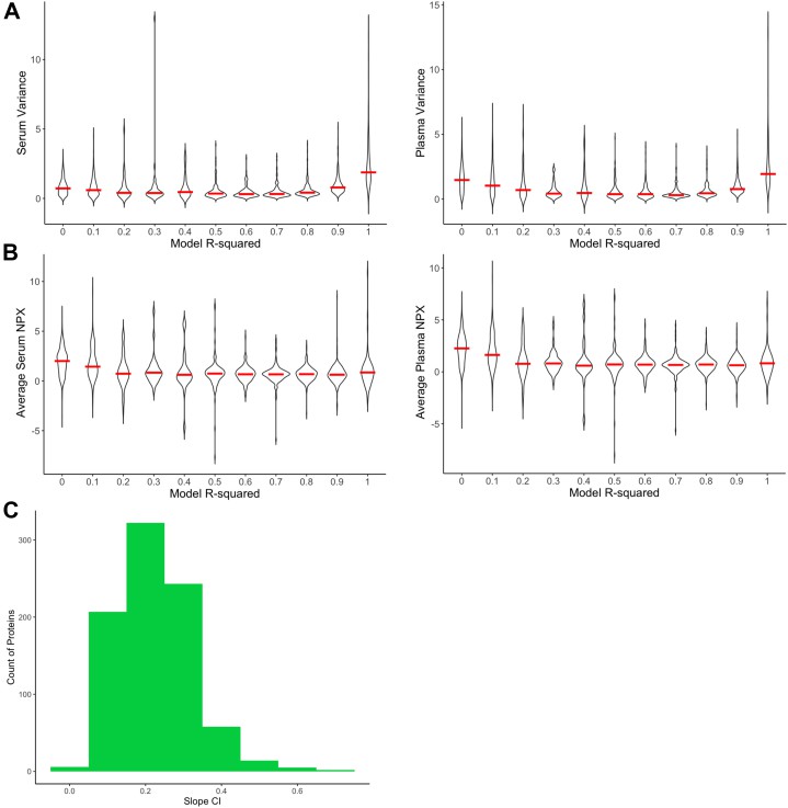
In a study titled "A Method for Comparing Proteins Measured in Serum and Plasma by Olink PEA Technology" authors analyzed matched serum and plasma from the same donors, using Explore and Target panels (~1,400 proteins). They found that many proteins have differing detectability depending on matrix, even after normalization and QC.
Key Takeaways:
- Some proteins had acceptable LOD in plasma but were below detection in serum, or vice versa.
- Batch-effect corrections and bridging were essential to align NPX distributions across sample types.
- Researchers reported that without accounting for matrix type in their statistical models, inferred differences could be confounded by matrix rather than biology.
How Interpretation Was Handled:
- They filtered proteins based on detectability thresholds in both matrices.
- Used paired statistical models to compare sample types.
- They emphasized fold changes together with confidence intervals and adjusted p-values, not just raw NPX differences.
Case Study B: High-Throughput Panel in Large Cohort for Biomarker Discovery
Another example is the UK Biobank Pharma Proteomics Project (UKB-PPP). They used Olink Explore panels on thousands of serum/plasma samples. Their workflow provides a strong model of how to deal with large datasets. Key features (from project documentation) include:
- Detailed QC: remove outliers, check assay precision (intra/inter-plate CVs), limit proteins with high missingness.
- Statistical modeling with covariates: age, sex, technical batch effects.
- Reporting of effect sizes, fold changes, and FDR adjustments.
Biological Insights:
- They discovered novel associations between genetic variants and protein expression (pQTLs).
- Some protein differences that seemed large in raw NPX narrowed after adjustment, showing importance of rigorous preprocessing.
Lessons for Your Interpretation Workflow
From these case studies, you should adopt these practices:
- Always filter for detectability across matrices or sample types.
- Model sample types or matrices explicitly if you have mixed serum/plasma.
- Report effect sizes + CI + adjusted p-values.
- Use large sample sizes or repeated measures whenever possible to increase statistical power.
- Where possible, validate findings with alternative methods (e.g. ELISA, mass spec) or independent cohorts.
Integrating Serum Proteomics with Other Omics & Clinical Data
To deepen biological understanding and improve robustness of findings, integrating Olink serum proteomics with other omics layers (transcriptomics, metabolomics, etc.) and relevant non-clinical phenotypic / sample metadata is extremely valuable. This section explains when and how to do that properly, with examples.
9.1 Why Multi-Omics Integration Strengthens Interpretations
Filling gaps in causality and regulation
mRNA levels often don't map directly onto protein abundance due to translation rates, post-translation modifications, and protein stability. Proteomics adds the layer reflecting closer to functional protein levels. Integrating with transcriptomics can reveal whether observed protein changes are driven at the transcriptional level, post-transcriptional regulation, or downstream regulation.
Metabolites as read-outs of protein function
Metabolomics captures small molecules downstream of enzyme activity. When a metabolic pathway shows both proteomic evidence (e.g. enzyme upregulation) and metabolite shifts, the confidence in biological mechanism is stronger.
Reducing false leads & increasing specificity
Signals that are supported by multiple omic layers are less likely to be artefacts. Combining omics helps prioritize biomarker candidates that are reproducible and more likely meaningful biologically.
9.2 What Data to Combine: Sample & Metadata Layers
When planning integration, consider combining:
| Data Type | Examples |
| Proteomics | Olink serum NPX values (after QC) |
| Transcriptomics | RNA-seq or microarray gene expression from matched samples, or public datasets |
| Metabolomics / Lipidomics | Small molecule profiling from same or biologically matched serum or tissue |
| Phenotypic / Sample Metadata | Age, sex, time point, treatment, collection site, storage, batch, clinical or exposure parameters (non-clinical) |
Matched sample sets (same individual / same time point) are ideal. If not possible, align as closely as possible (e.g. same cohort, same treatment, similar sample handling).
9.3 Integration Strategies & Analytical Methods
Correlation networks / co-expression / co-abundance analysis
Compute correlation or partial correlation between transcript levels and protein NPX, or between proteins and metabolites. Identify modules (clusters) of co-regulated entities. For example, genes highly correlated with serum proteins may indicate upstream regulators.
Over-representation / joint pathway enrichment
Use pathway databases (Reactome, GO, KEGG) to test which pathways are enriched both in proteomic and transcriptomic or metabolomic differential results. Joint enrichment strengthens the evidence.
Multivariate / dimension reduction methods
Methods like canonical correlation analysis (CCA), partial least squares (PLS), or multiblock PLS allow integrating two or more datasets to find components that explain co-variation.
Machine learning models using multi-omics features
In non-clinical settings, these models can help classify sample conditions, or correlate omics features with exposure or phenotype. But always guard against overfitting (use cross-validation, independent test sets).
Single-sample or paired workflows
When possible, process the same sample for multiple omics. For example, using workflows where metabolites are extracted first, and the residual protein is used for proteomics, reducing pre-analytic noise. A recent study (MTBE-SP3) did this for metabolomics + proteomics on serum/plasma, showing consistent proteomic profiles irrespective of metabolite extraction method. (Gegner et al., 2024. DOI: https://doi.org/10.1186/s12014-024-09501-9)
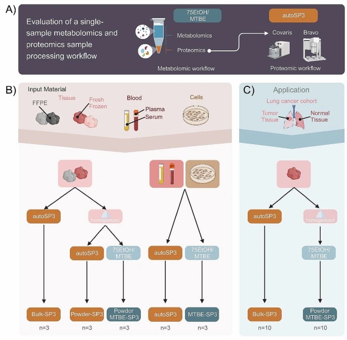 Overview of experimental setup.
9.4 Example: Olink + Transcriptomics Integration
A recently published study "The Integration of Olink Proteomics with Transcriptomics Elucidates …" used Olink's Inflammation Panel on conditioned media (after TNF-α stimulation) along with transcriptomics (mRNA) from the same treated cells. They demonstrated which inflammatory proteins corresponded with upregulated transcripts, and which did not—allowing insight into post-transcriptional regulation. (Study published in 2025)
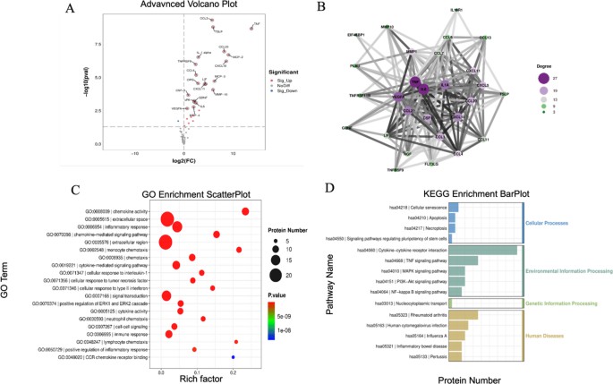 All differentially expressed inflammation-related and bioinformatics analysis.
This example underscores:
- The value of matching cell/tissue/condition for both omics.
- Adjusting for technical variation in each dataset separately before integration.
- Considering proteins that diverge from mRNA fold changes as candidates for regulation or modification.
9.5 Practical Tips & Considerations for Integrative Analysis
Ensure matching / alignment of samples and metadata
Time point, sample handling, storage, experimental condition must be matched or well documented. Misalignment confounds interpretation.
Deal with missingness separately in each omic layer
Proteomic missingness (below LOD) and transcriptomic dropouts or low expression both need filtering or imputation appropriate to that layer.
Scaling and normalization
After QC, normalize each omic dataset appropriately (e.g. transcript counts normalized, NPX normalized, metabolite abundances normalized). Consider dimension reduction after per-omic normalization.
Batch effects across omics
Different omics layers may have different batch variables (e.g. sequencing batch vs proteomics plate). Model them separately and, when possible, include batch covariates.
Choice of integration tools
- Some tools/libraries useful in multi-omics integration:
- mixOmics (R) for PLS/CCA-based methods and visualization.
- Pathway enrichment tools that accept multi-omics input.
- Network tools to build correlation or regulatory networks.
Interpretation cautious of overclaim
Because multiple layers increase complexity, avoid overclaiming causality. Use integration to generate hypotheses; validation is still needed (e.g. via orthogonal assays or separate cohorts).
How Interpreting Serum Results Differs from Plasma / Other Matrices
When using Olink serum proteomics panels, it's important to recognise that serum is not equivalent to plasma (or other matrices) in detectability, variability, and baseline behaviour. Misunderstanding these differences can lead to misinterpretation of results. Here are what is known, what to watch out for, and strategies to adjust.
10.1 Key Differences Between Serum vs Plasma
Proteolytic activity during clotting
Serum is produced after blood clots. During clot formation and subsequent processing, proteases may be activated and cause degradation or modification of some proteins. This can reduce detectability or shift NPX values. (See Determination of temporal reproducibility and variability… using the Olink I-O panel; many proteins had differing serum:plasma ratios.
Anticoagulant effects, residual fibrin, and clotting artefacts
Plasma (e.g. EDTA plasma) suppresses clotting; hence anticoagulants prevent protease activation. Serum, lacking these, may have residual clotting‐associated factors (fibrin, platelets) that affect background or interfere with some assays differently.
Baseline abundance & detectability
Some proteins are more easily detected in plasma than serum. For example, in a study of over 1,100 paired serum/plasma samples for predicting gestational age, plasma signatures had higher predictive power than serum. Serum proteins often had weaker association strength.
Quantitative differences / transformation factors
In the paper "A Method for Comparing Proteins Measured in Serum and Plasma…" ~1,463 proteins were measured; many required transformation factors to align serum and plasma results. Some proteins differed substantially (higher or lower NPX in serum vs plasma) even after normalization.
Reproducibility & inter-study / inter-assay variation
In the I-O panel study (paired serum and EDTA plasma), reproducibility varied. For about half the proteins, serum vs plasma measurement ratios were consistent; for others they were not (poor correlation or high variability), making some proteins unreliable across matrices.
10.2 What These Differences Mean for Interpretation
You cannot directly compare NPX values from serum vs plasma for the same protein without adjustment. A difference you attribute to biology may actually be a matrix effect.
When combining datasets, if one uses plasma and another uses serum, the observed differences might partly reflect matrix biases rather than true biological variation.
Some proteins may be "lost" or under-quantified in serum because of degradation or lower detectability. That can bias downstream pathway analysis if low-abundance proteins disproportionately drop out.
Associations or predictive models developed in plasma may not translate equally well to serum, and vice versa. Predictive power and effect size may differ. (E.g. gestational age prediction in Espinosa et al.)
10.3 Best Practices to Handle Matrix Differences
Use paired samples where possible
If you expect to compare serum vs plasma (or move between matrices), collect matched serum + plasma from the same individual(s) and time point. That allows you to compute transformation factors or at least assess how each protein behaves across matrices.
Include matrix type as a covariate in statistical models
When analysing data, explicitly include "matrix" (serum vs plasma) in your regression or mixed effects models. That helps adjust for baseline shifts or detectability differences.
Apply transformation factors / normalization between matrices
Use published transformation factors to adjust NPX values when possible. The Comparing Proteins Measured in Serum and Plasma… study generated many such factors for hundreds of proteins.
Filter proteins by detectability in both matrices
Remove or downweight proteins that are reliably measured (above LOD and acceptable variance) only in one matrix. If a protein is only detectable in plasma but often below LOD in serum, be cautious about interpreting changes in serum data.
QC checks separately for each matrix
Internal controls, CVs, plate controls may behave differently in serum vs plasma. Always compute QC metrics within the matrix, and inspect sample-specific flags. (The I-O study showed mean serum-plasma ratios varying notably for some proteins; variability pre- and post-normalization was significant.
10.4 Case Examples Illustrating Matrix Effects
In "Determination of temporal reproducibility and variability…" (I-O panel, serum vs EDTA plasma), out of 92 proteins:
Approx. 80 proteins were evaluable for matrix comparison.
For many proteins, the serum:plasma ratio ranged from ~0.41 to ~3.01, meaning serum NPX could be less than half—or more than three times—plasma NPX.
36 proteins showed poor comparability due to high ratio variability or correlation issues.
In the gestational age prediction study (73 women, 1,116 proteins, paired serum/plasma), plasma signatures had markedly higher correlation (R ≈ 0.64) vs serum (R ≈ 0.45) for predicting gestational age. When serum signature was validated in plasma, predictive power held moderately; but plasma → serum was weaker.
Recommendations & Best Practices Checklist
Here is a distilled checklist of best practices you should follow when interpreting results from Olink serum proteomics. Use it as a guide or SOP add-on to help ensure your data is high quality, your interpretations are robust, and your conclusions are credible.
Best Practices Checklist
| Step | What to Do | Why It Matters |
| 1. Sample collection & handling | - Use consistent Type & brand of collection tubes. - Allow clotting time in serum: 15-30 min at room temp; avoid >60 min. - Centrifuge at 2-8 °C, ~10 min, ~1,000-2,000 × g. - Aliquot and freeze at −80 °C; avoid multiple freeze-thaws. - Transport frozen on dry ice; use non-protein binding containers. |
Minimises variation, proteolysis, and aberrant NPX shifts. Creative-Proteomics' protocol emphasises these handling details. |
| 2. Sample metadata & randomization | - Record sample metadata: donor, collection time, storage duration, batch, site. - Randomize case/control samples across plates/runs. - Include matrix (serum vs plasma) where mixed. |
Helps adjust for non-biological variation and avoid confounding. |
| 3. Include and monitor QC controls | - Use Olink internal controls per sample: incubation, detection, extension controls. - Include external controls: sample control (pooled), negative, calibrator. - Use inter-plate controls (IPC) if running multiple plates. - Examine exactly which QC flags are triggered; don't ignore warnings. |
Without QC, technical artefacts dominate. E.g. |
| 4. Detect outliers early | - Use PCA, MDS, or clustering to identify samples far from others. - Plot NPX distributions per sample and per protein; check IQR, median. - Remove or flag problematic samples before major analysis. |
Outliers distort group means and fold-change estimates. |
| 5. Filter on detection frequency & LOQ/LOD | - Exclude proteins with >50 % (or some cutoff) of samples below LOD or LOQ. - Treat values below LOD with care: impute or flag, consider sensitivity analyses. - Report number of proteins remaining post-filtering. |
Helps avoid false discoveries driven by noise. UK Biobank and other large-cohort studies follow this practice. |
| 6. Normalize and bridge when needed | - Use IPC or external calibrators to adjust for plate effects. - If combining batches or matrices, use bridge samples and compute transformation factors (see serum vs plasma study). - Choose a reference dataset for alignment. |
Ensures comparability; avoids artefactual differences across plates or sample types. |
| 7. Choose appropriate statistical methods | - Check whether data meet parametric test assumptions; otherwise use non-parametric or mixed models. - Include covariates (batch, matrix, donor metadata). - Control for multiple testing (FDR) and report adjusted p-values. - Always report effect sizes with confidence intervals. |
Helps balance detecting real signals and avoiding false positives. |
| 8. Biological interpretation and pathway analyses | - Ensure background/universe for enrichment is appropriate (measured proteins post-QC). - Use ORA or GSEA and verify literature support. - Integrate with other omics or metadata if available to strengthen hypotheses. |
Prevents overclaiming, improves biological insight. |
| 9. Document every decision | - Keep a log: which samples were excluded, why; what normalization chosen; which covariates used; any imputation / handling of low signals. - Keep software versions, panel versions, QC thresholds noted. |
Ensures reproducibility within lab and transparency for readers / reviewers. |
| 10. Validate key findings if possible | - Use orthogonal methods (e.g. ELISA, mass spec) for candidate proteins. - Try replication in independent cohorts if available. - Confirm whether findings hold under different sample matrices. |
Adds confidence, especially for biomarker discovery or mechanistic studies. |
Additional Recommended Practices
Power calculation: Before beginning large studies, estimate how many samples you need to detect expected effect sizes with desired power. Olink's white paper on biomarker study design provides methods.
Consult vendor / community resources: Use Olink's technical notes, validation data, and white papers to stay up to date.
Use software pipelines built for Olink data: E.g. OlinkAnalyze R package, or maintained tools like „Omics Playground" for QC-aware analysis of Olink NPX data.
Actionable Next Steps & Call to Action
You've now seen how to interpret Olink serum proteomics results in depth. To turn insight into impact, below are concrete, actionable steps you can take right away, plus suggestions for how we can help you move forward.
What You Can Do Now
Set up your data pipeline using OlinkAnalyze
- Install the latest version of OlinkAnalyze (version 4.3.1 as of July 31, 2025) from CRAN or its R-Universe repo.
- Use provided vignettes for LOD computation, bridging, outlier exclusion, and normalization.
Audit your past or current projects for pitfalls
Review whether sample handling was consistent (clotting, freeze-thaw cycles).
Check whether QC flags were ignored, or batches/plates were treated properly.
Re-evaluate whether NPX differences were interpreted correctly (i.e. not comparing across proteins or matrices without adjustment).
Integrate additional metadata or omics layers
- If you have matching transcriptomics, metabolomics, or exposure data, try correlating those with differential proteins.
- Make sure sample metadata (batch, matrix, donor info) is complete and included in models.
Filter and validate candidate proteins
- Apply detection-frequency and LOD filtering.
- For top candidates, validate using an orthogonal method (e.g. ELISA, mass spectrometry) or replicate in a second cohort.
- Check effect sizes + confidence intervals; don't rely purely on p-value or NPX difference.
Document everything for reproducibility
- Keep versioned logs of data preprocessing steps, QC metrics, normalization choices, statistical models used.
- Save code snippets (e.g. OlinkAnalyze pipelines), parameter settings, and make them shareable within your team or with collaborators.
How We Can Help You
If you prefer expert support or want to accelerate your results with high confidence, here's how our services align with your needs:
Service design & assay setup: We help define the best Olink panel(s) for your research question, plan experiments to maximize detectability and reduce variation.
Data analysis & interpretation support: Using our experience with Olink NPX workflows, we can process your raw NPX data through QC, normalization, bridging, statistical testing, and biological interpretation.
Visualization & reporting: We can generate publication-quality figures (volcano plots, heatmaps, pathway maps), with clear annotations of effect size and statistical metrics.
Integration projects: If you have omics layers (transcriptomics, metabolomics, etc.), we support integration workflows, cross-validation, and network/pathway analysis to strengthen findings.
References
- Shraim R, Diorio C, Canna SW, Macdonald-Dunlop E, Bassiri H, Martinez Z, Mälarstig A, Abbaspour A, Teachey DT, Lindell RB, Behrens EM. A Method for Comparing Proteins Measured in Serum and Plasma by Olink Proximity Extension Assay. Mol Cell Proteomics. 2025
- Pascovici D, Handler DC, Wu JX, Haynes PA. Multiple testing corrections in quantitative proteomics: A useful but blunt tool. Proteomics. 2016 Sep;16(18):2448-53. doi: 10.1002/pmic.201600044. PMID: 27461997.
- Gegner, H.M., Naake, T., Aljakouch, K. et al. A single-sample workflow for joint metabolomic and proteomic analysis of clinical specimens. Clin Proteom 21, 49 (2024).
- Zhou, Y., Xiao, J., Peng, S. et al. The Integration of Olink Proteomics with Transcriptomics Elucidates that TNF-α Induces Senescence and Apoptosis in Transplanted Mesenchymal Stem Cells. Stem Cell Rev and Rep 21, 2298–2309 (2025).
- Heckendorf C, Blum BC, Lin W, Lawton ML, Emili A. Integration of Metabolomic and Proteomic Data to Uncover Actionable Metabolic Pathways. Methods Mol Biol. 2023;2660:137-148. doi: 10.1007/978-1-0716-3163-8_10. PMID: 37191795.


